National Science Foundation Grant Terminations under the Trump Administration

library(dplyr)
library(tidyr)
library(stringr)
library(curl)
library(ggplot2)
library(ggimage)
library(ggrepel)
library(ggtext)
  

# ---- Data Preparation ----

tuesdata <- tidytuesdayR::tt_load(2025, week = 14)
care_state <- tuesdata$care_state

data2plot <- 
  care_state |>
  mutate(score = if_else(is.na(score), 0, score)) |>
  filter(measure_id %in% c('HCP_COVID_19','IMM_3')) |>
  mutate(measure_id = case_when(
    measure_id == 'HCP_COVID_19' ~ "COVID-19",
    measure_id == 'IMM_3' ~ "Influenza"
  ))

# --- Raw Plot
data2plot |>
  ggplot(aes(x = score, y = state, fill = measure_id)) +
  geom_col()

# --- Stage 2

library(geofacet)
data2plot |>
  ggplot(aes(x = score, y = measure_id)) +
  geom_col(aes(fill = measure_id)) +
  facet_geo(~ state, grid = "us_state_grid1", strip.position = "top")

# --- Stage 3

data2plot |>
  ggplot(aes(x = score, y = measure_id)) +
  geom_col(aes(fill = measure_id)) +
  facet_geo(~ state, grid = "us_state_grid1", strip.position = "top") +
  coord_polar() +
  geom_text(data = .%>% filter(measure_id == 'Influenza'), x = 0, y = -1, aes(label = scales::percent(score/100, accuracy = 1), color = measure_id), size = 2.5,fontface = "bold") +
  geom_text(data = .%>% filter(measure_id == 'COVID-19'), x = 0, y = -3, aes(label = scales::percent(score/100, accuracy = 1), color = measure_id), size = 2.5,fontface = "bold") +
  scale_y_discrete(expand = c(0,3,0,0)) +
  scale_x_continuous(limits = c(0,100), expand = c(0,0,0,0)) +
  theme_void()

# --- Stage 4

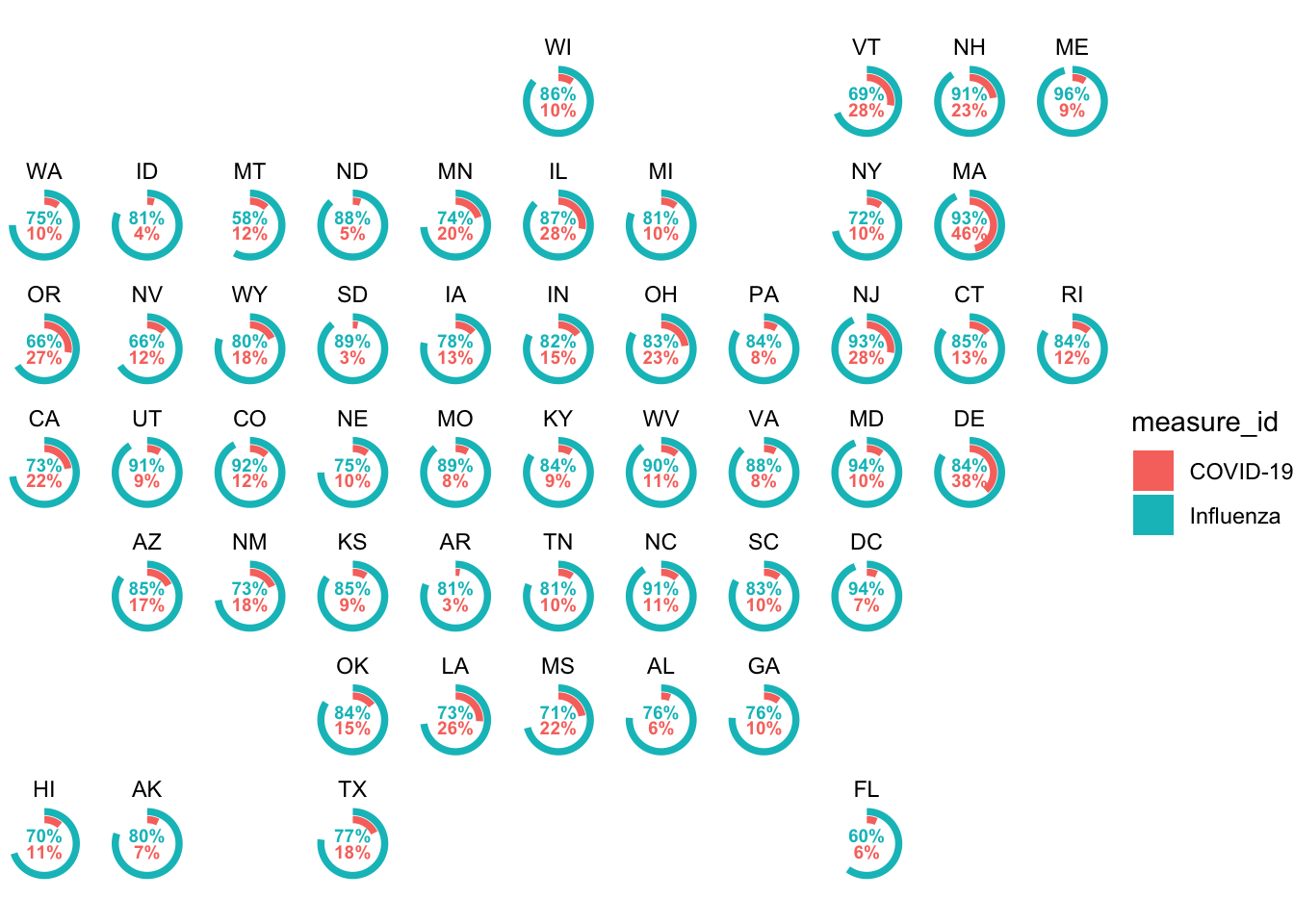
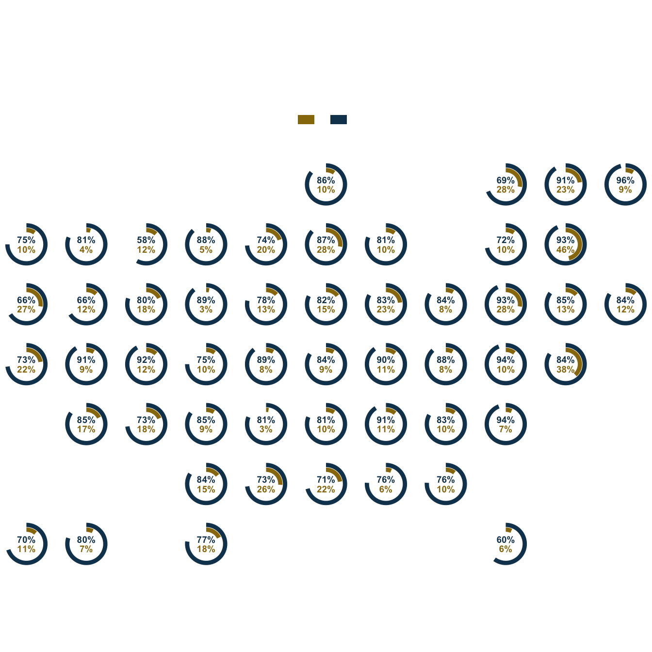
data2plot |>
  ggplot(aes(x = score, y = measure_id)) +
  geom_col(aes(fill = measure_id)) +
  geom_text(data = .%>% filter(measure_id == 'Influenza'), x = 0, y = -1, aes(label = scales::percent(score/100, accuracy = 1), color = measure_id), size = 2.5,fontface = "bold") +
  geom_text(data = .%>% filter(measure_id == 'COVID-19'), x = 0, y = -3, aes(label = scales::percent(score/100, accuracy = 1), color = measure_id), size = 2.5,fontface = "bold") +
  coord_polar() +
  facet_geo(~ state, grid = "us_state_grid1", strip.position = "top") +
  scale_y_discrete(expand = c(0,3,0,0)) +
  scale_x_continuous(limits = c(0,100), expand = c(0,0,0,0)) +
  scale_fill_manual(values = c("#99780b","#14405C")) +
  scale_color_manual(values = c("#99780b","#14405C")) +
  labs(
    fill = NULL, 
    title = "US Healthcare Personnel Vaccination", 
    subtitle = "Percentage of healthcare personnel who are up to date with COVID-19 or Influenza vaccinations on US (2024)",
    caption = 'SOURCE: #Tidytuesday 2025-04-08') +
  guides(color = 'none') +
  theme_void() +
  theme(
    plot.title.position = "plot",
    plot.title = element_text(family = "Ubuntu", size = 20, face = 'bold'),
    plot.subtitle = element_markdown(size = 9,lineheight = 1.25, margin = margin(5,0,20,0)),
    legend.position = "top",
    text = element_text(family = "Ubuntu"),
    strip.text = element_text(color = 'grey30'),
    legend.margin = margin(0,0,20,0),
    legend.spacing = unit(0.1, 'cm'),
    legend.key.height= unit(0.3, 'cm'),
    legend.key.width= unit(0.5, 'cm'))