Seismic Events at Mount Vesuvius – TidyTuesday by Rodrigo

About the Data

Note

Check data in tidytuesday GitHub repository.

The dataset this week explores seismic events detected at the famous Mount Vesuvius in Italy. It comes from the Italian Istituto Nazionale di Geofisica e Vulcanologia (INGV)’s Data Portal and can be explored along with other seismic areas on the GOSSIP website. The raw data was saved as individual CSV files from the GOSSIP website and some values were translated from Italian to English.

The Open Data Portal of Istituto Nazionale di Geofisica e Vulcanologia (INGV) gives public access to data resulting from institutional research activities in the fields of Seismology, Volcanology, and Environment.

1 Initializing

1.1 Load libraries

library(tidyverse)
library(glue)
library(scales)
library(showtext)
library(ggtext)
library(shadowtext)
library(hexbin)
library(OpenStreetMap)
library(ggplot2)
library(ggspatial)
library(sf)
library(ggforce)

font_add_google("Ubuntu", "Ubuntu", regular.wt = 400, bold.wt = 700)
showtext_auto()
showtext_opts(dpi = 300)

1.2 Set theme

theme_set(
    theme_minimal() +
    theme(
    axis.line.x.bottom = element_line(color = '#47506e', linewidth = .3),
    # axis.ticks.x= element_line(color = '#47506e', linewidth = .3),
    axis.line.y.left = element_line(color = '#47506e', linewidth = .3),
    # axis.ticks.y= element_line(color = '#47506e', linewidth = .3),
    panel.grid = element_line(linewidth = .3, color = '#aebae0'),
    panel.grid.minor = element_blank(),
    axis.ticks.length = unit(-0.15, "cm"),
    plot.background = element_blank(),
    plot.title.position = "plot",
    plot.title = element_text(family = "Ubuntu", size = 18, face = 'bold'),
    plot.caption = element_text(size = 8, color = '#aebae0',margin = margin(20,0,0,0)),
    plot.subtitle = element_text(size = 9,lineheight = 1.15, margin = margin(5,0,15,0)),
    axis.title.x = element_markdown(family = "Ubuntu", hjust = .5, size = 8, color = "#47506e"),
    axis.title.y = element_markdown(family = "Ubuntu", hjust = .5, size = 8, color = "#47506e"),
    axis.text = element_text(family = "Ubuntu", hjust = .5, size = 8, color = "#47506e"),
    legend.position = "top",
    text = element_text(family = "Ubuntu"),
    plot.margin = margin(25, 25, 25, 25))
)

1.3 Load this week’s data

tuesdata <- tidytuesdayR::tt_load(2025, week = 19)
vesuvius <- tuesdata$vesuvius

2 Data analysis

How many events per year

vesuvius |> mutate(year = year(time)) |> count(year) |> ggplot(aes(x = year, y = n)) + geom_col() + theme_minimal()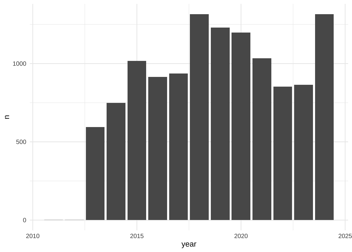

vesuvius |> mutate(year = year(time)) |> group_by(year) |> summarize(md = mean(duration_magnitude_md, na.rm = TRUE)) |> ungroup() |> ggplot(aes(x = year, y = md)) + geom_col() + theme_minimal()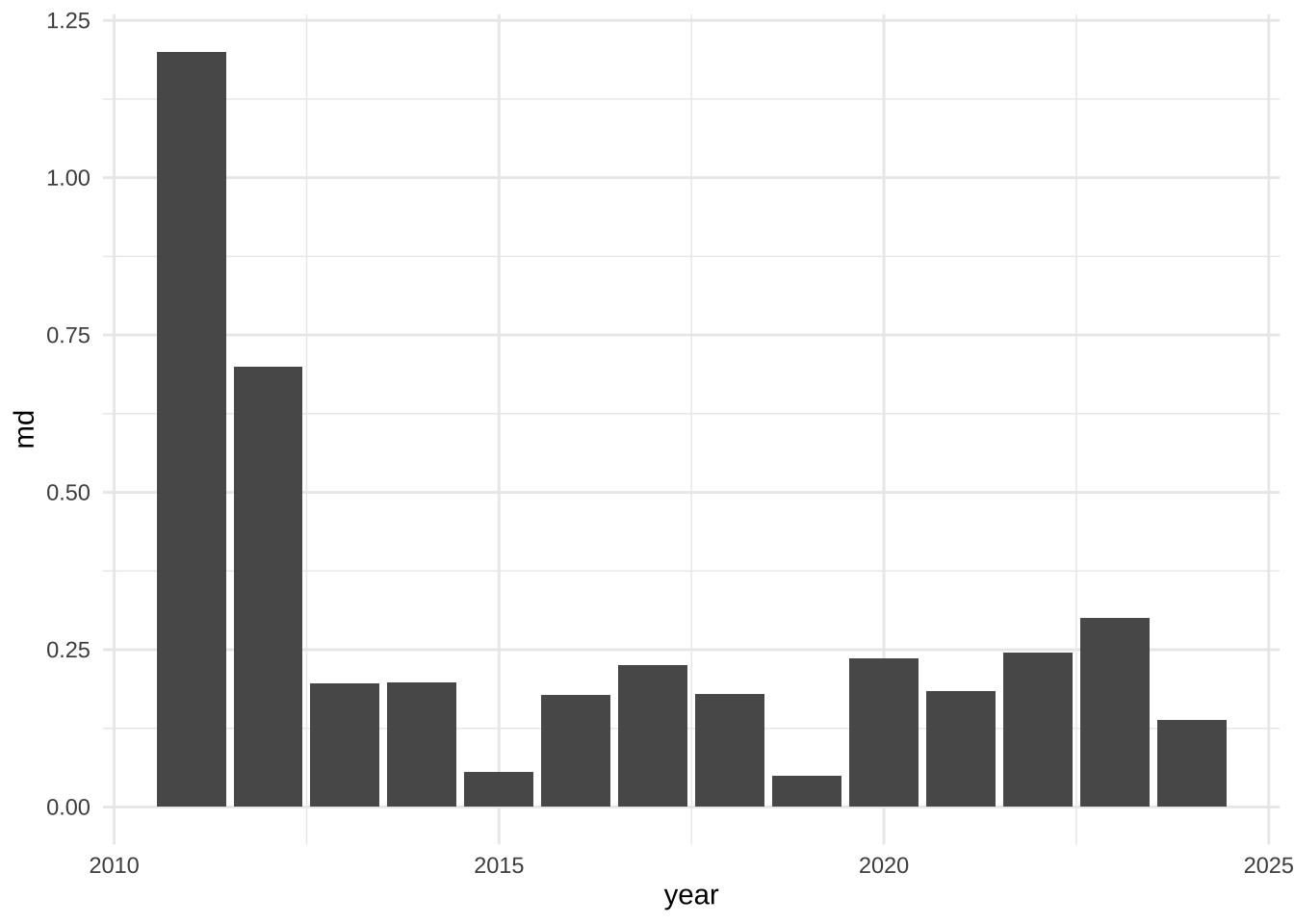

Geo distribuiton

vesuvius |> mutate(year = year(time)) |> ggplot(aes(x = latitude, y = longitude)) + geom_point(aes(color = time)) + theme_minimal()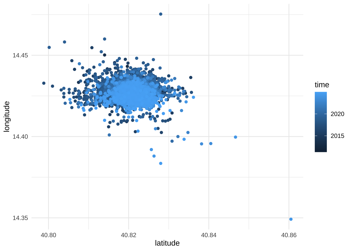

vesuvius |> mutate(year = year(time)) |> filter(year == max(year)) |> ggplot(aes(x = latitude, y = longitude)) + 
  geom_point(aes(color = time)) + theme_minimal()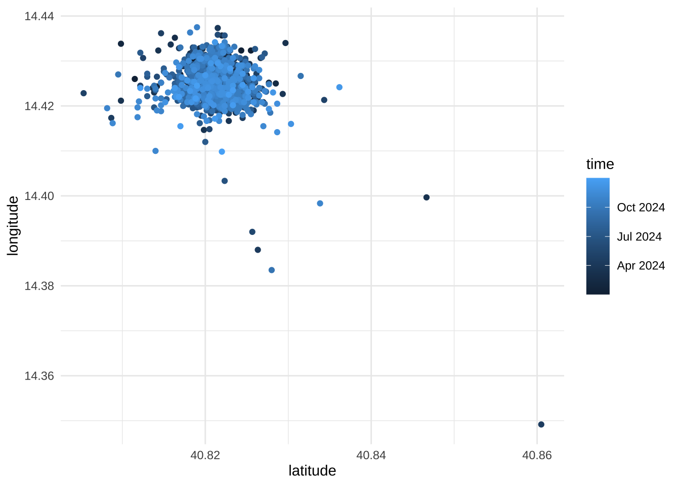

3 Transform Data for Plotting

3.1 Calculate counts by hex bin

At the beggining I was trying to use the defaul ggplot hexbin, but it can’t change size so I have to calculate my own.

data2plot <- vesuvius |>
  mutate(year = year(time)) |>
  filter(year == max(year), longitude > 14.405)

hb_counts <- hexbin::hexbin(
  data2plot$latitude,
  data2plot$longitude,
  xbins = 20,
  IDs = TRUE
)

hex_summary_counts <- data.frame(
  hcell2xy(hb_counts),
  count = hb_counts@count # Accesses the count for each bin
)

3.2 Loading Map

my_data_sf <- st_as_sf(hex_summary_counts, coords = c("x", "y"), crs = 4326)
my_data_transformed <- st_transform(my_data_sf, crs = 3857)
extent <- st_bbox(my_data_transformed)

open_map <- openmap(
  upperLeft = c(
    min(hex_summary_counts$x) - .0025,
    max(hex_summary_counts$y) + .0025
  ),
  lowerRight = c(
    max(hex_summary_counts$x) + .0025,
    min(hex_summary_counts$y) - .0025
  ),
  zoom = NULL,
  mergeTiles = TRUE,
  type = "bing",
  minNumTiles = 10
)
sa_map2 <- openproj(open_map)

4 Time to plot!

4.1 Before

vesuvius |>
  mutate(year = year(time)) |>
  filter(year == max(year), longitude > 14.405) |>
  ggplot(aes(x = latitude, y = longitude)) +
  geom_hex(
    binwidth = c(.0012),
    aes(linewidth = after_stat(count)),
    color = 'white'
  ) +
  theme_minimal() +
  coord_fixed() +
  scale_linewidth(range = c(1.5, 0)) +
  scale_fill_distiller(palette = "Spectral")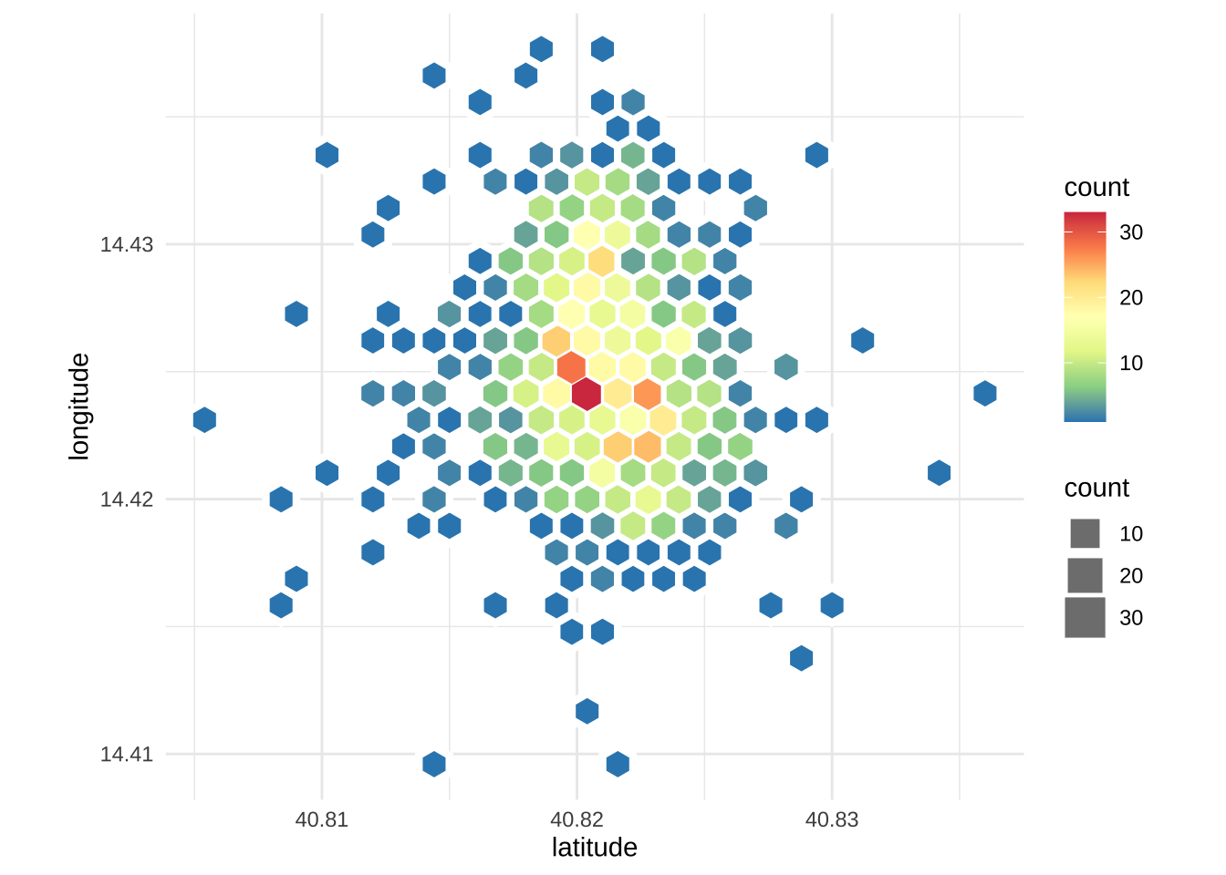

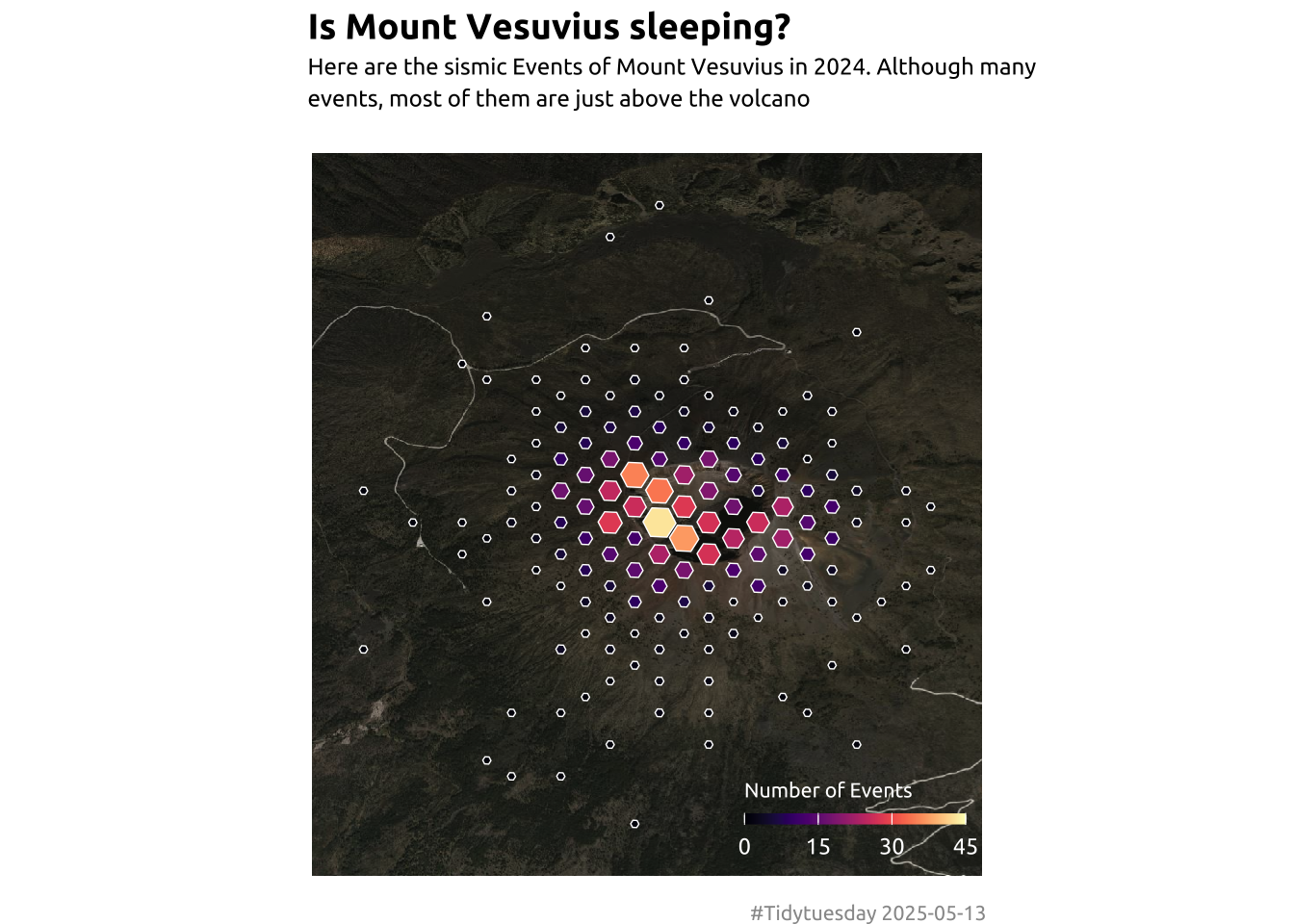
4.2 After

OpenStreetMap::autoplot.OpenStreetMap(sa_map2) +
  ggforce::geom_regon(
    data = hex_summary_counts,
    aes(
      x0 = y,
      y0 = x,
      sides = 6,
      r = scales::rescale(count, to = c(0.0002, 0.0008)),
      angle = 1,
      fill = count,
    ),
    alpha = 1,
    # color = '#441C77',
    color = 'white',
    size = .25
  ) +
  scale_size(range = c(0.5, 3)) +
  theme_void() +
  viridis::scale_fill_viridis(
    option = 'magma',
    breaks = seq(0, 45, 15),
    limits = c(0, 45)
  ) +
  labs(
    title = 'Is Mount Vesuvius sleeping?',
    subtitle = str_wrap(
      width = 70,
      "Here are the sismic Events of Mount Vesuvius in 2024. Although many events, most of them are just above the volcano"
    ),
    fill = "Number of Events",
    caption = "#Tidytuesday 2025-05-13"
  ) +
  theme(
    strip.background = element_blank(),
    strip.text = element_blank(),
    text = element_text(family = "Ubuntu"),
    plot.title.position = "plot",
    plot.title = element_text(family = "Ubuntu", size = 14, face = 'bold'),
    plot.caption = element_text(
      size = 8,
      color = 'grey60',
      margin = margin(10, 0, 0, 0)
    ),
    legend.title = element_text(size = 8, color = 'white'),
    legend.justification = c(1, 0),
    legend.position = c(0.97, 0.03),
    legend.direction = 'horizontal',
    legend.text = element_text(color = 'white'),
    plot.subtitle = element_text(
      size = 9,
      lineheight = 1.15,
      margin = margin(5, 0, 15, 0)
    )
  ) +
  guides(
    fill = guide_colorbar(
      barwidth = 6,
      barheight = .3,
      title.position = 'top'
    )
  )