Project Gutenberg – TidyTuesday by Rodrigo

About the Data

Note

Check data in TidyTuesday GitHub repository.

This week we’re exploring books from Project Gutenberg and the {https://docs.ropensci.org/gutenbergr/} R package!

[{gutenbergr} allows you to] Download and process public domain works in the Project Gutenberg collection https://www.gutenberg.org/. Includes metadata for all Project Gutenberg works, so that they can be searched and retrieved.

1 Initializing

1.1 Load libraries

library(tidyverse)
library(glue)
library(scales)
library(showtext)
library(ggtext)
library(shadowtext)

font_add_google("Ubuntu", "Ubuntu", regular.wt = 400, bold.wt = 700)
showtext_auto()
showtext_opts(dpi = 300)

1.2 Set theme

theme_set(
    theme_minimal() +
    theme(
    # axis.line.x.bottom = element_line(color = '#474747', linewidth = .3),
    # axis.ticks.x= element_line(color = '#474747', linewidth = .3),
    # axis.line.y.left = element_line(color = '#474747', linewidth = .3),
    # axis.ticks.y= element_line(color = '#474747', linewidth = .3),
    # # panel.grid = element_line(linewidth = .3, color = 'grey90'),
    panel.grid.major = element_blank(),
    panel.grid.minor = element_blank(),
    axis.ticks.length = unit(-0.15, "cm"),
    plot.background = element_blank(),
    plot.title.position = "plot",
    plot.title = element_text(family = "Ubuntu", size = 18, face = 'bold'),
    plot.caption = element_text(size = 8, color = 'grey60',margin = margin(20,0,0,0)),
    plot.subtitle = element_text(size = 9,lineheight = 1.15, margin = margin(5,0,15,0)),
    axis.title.x = element_markdown(family = "Ubuntu", hjust = .5, size = 8, color = "grey40"),
    axis.title.y = element_markdown(family = "Ubuntu", hjust = .5, size = 8, color = "grey40"),
    axis.text = element_text(family = "Ubuntu", hjust = .5, size = 8, color = "grey40"),
    legend.position = "top",
    text = element_text(family = "Ubuntu", color = "#495373"),
    plot.margin = margin(25, 25, 25, 25))
)

1.3 Load this week’s data

tuesdata <- tidytuesdayR::tt_load(2025, week = 22)

gutenberg_authors <- readr::read_csv('https://raw.githubusercontent.com/rfordatascience/tidytuesday/main/data/2025/2025-06-03/gutenberg_authors.csv')
gutenberg_languages <- readr::read_csv('https://raw.githubusercontent.com/rfordatascience/tidytuesday/main/data/2025/2025-06-03/gutenberg_languages.csv')
gutenberg_metadata <- readr::read_csv('https://raw.githubusercontent.com/rfordatascience/tidytuesday/main/data/2025/2025-06-03/gutenberg_metadata.csv')
gutenberg_subjects <- readr::read_csv('https://raw.githubusercontent.com/rfordatascience/tidytuesday/main/data/2025/2025-06-03/gutenberg_subjects.csv')

2 Data analysis

How many types are languages?

gutenberg_languages |> count(language, sort = TRUE)

# A tibble: 70 × 2
   language     n
   <chr>    <int>
 1 en       60693
 2 fr        3973
 3 fi        3313
 4 de        2324
 5 it        1056
 6 nl        1046
 7 es         885
 8 pt         647
 9 hu         609
10 zh         444
# ℹ 60 more rows

How many authors are there?

gutenberg_authors |> count(author, sort = TRUE)

# A tibble: 25,940 × 2
   author                n
   <chr>             <int>
 1 Hughes, Thomas        4
 2 Smith, George         4
 3 Taylor, Thomas        4
 4 Wilson, John          4
 5 Anderson, William     3
 6 Brown, John           3
 7 Brown, Thomas         3
 8 Butler, Samuel        3
 9 Edwards, Edward       3
10 Fowler, Frank         3
# ℹ 25,930 more rows

Repeated author names? (Coincidence?)

3 Transform Data for Plotting

3.1 Creating table of authors with most records for each language

author_blocklist <- c('Various', 'Anonymous', 'Unknown', NA)

data2plot <-
  gutenberg_metadata |>
  select(gutenberg_author_id, language) |>
  left_join(gutenberg_authors, by = 'gutenberg_author_id') |>
  count(gutenberg_author_id, author, language, sort = TRUE) |>
  filter(!author %in% author_blocklist) |>
  group_by(language) |>
  slice_max(n = 1, order_by = n, with_ties = FALSE) |>
  ungroup() |>
  arrange(-n) |>
  head(10)


data2plot <- bind_rows(
  data2plot |> mutate(to_dodge = TRUE),
  data2plot |> mutate(to_dodge = FALSE))

data2plot <- data2plot |> mutate(label = glue('**{author}**<span style="color:#aebae0"> {language}</span>'))

4 Time to plot!

4.1 Before

data2plot |> filter(to_dodge) |>
  ggplot(aes(x = n, y = author)) +
  geom_col() +
  theme_gray() +
  labs(
    title = 'Language Favorites',
    subtitle = 'Authors in Project Gutenberg with most records for the top 10 languages.')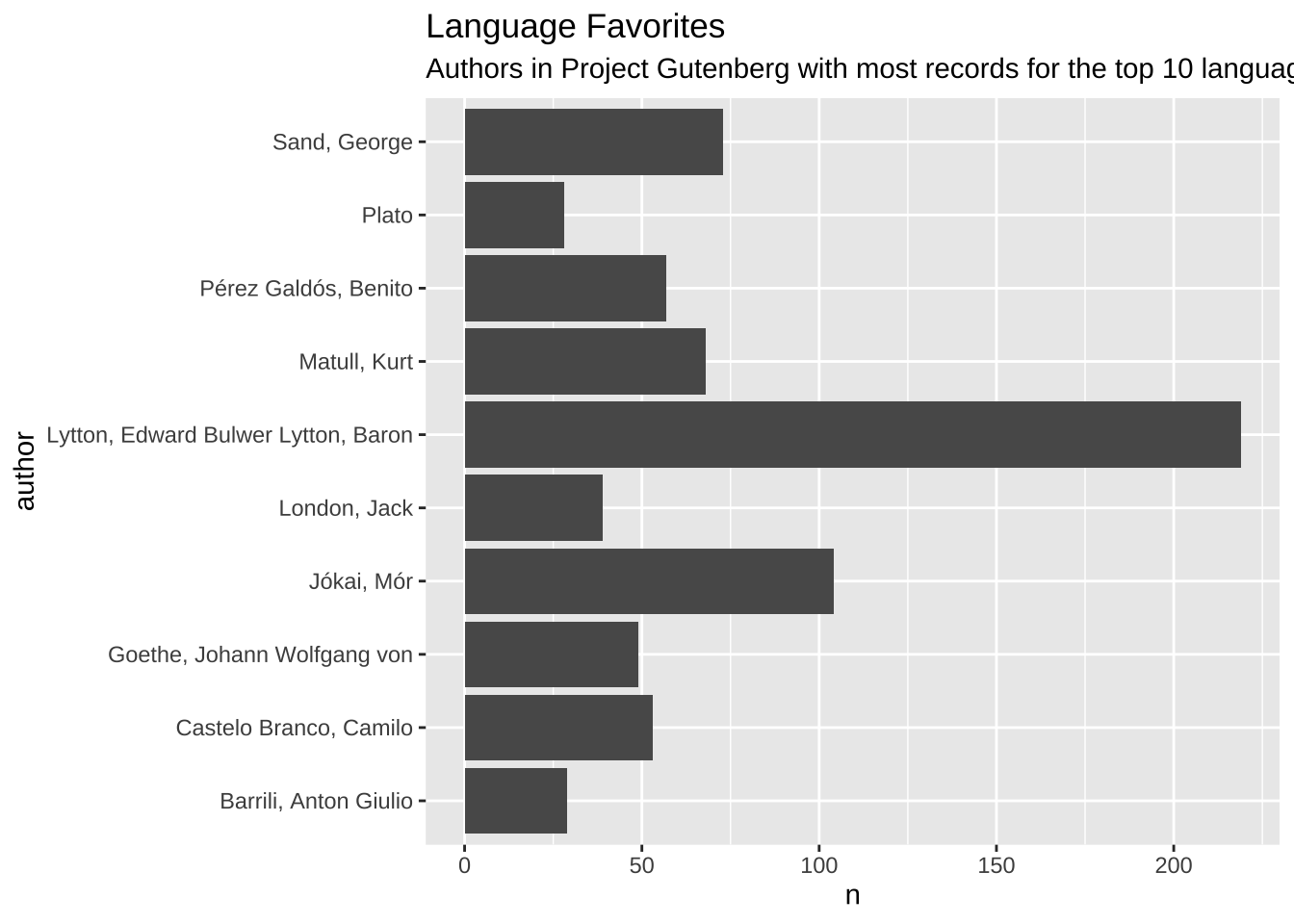

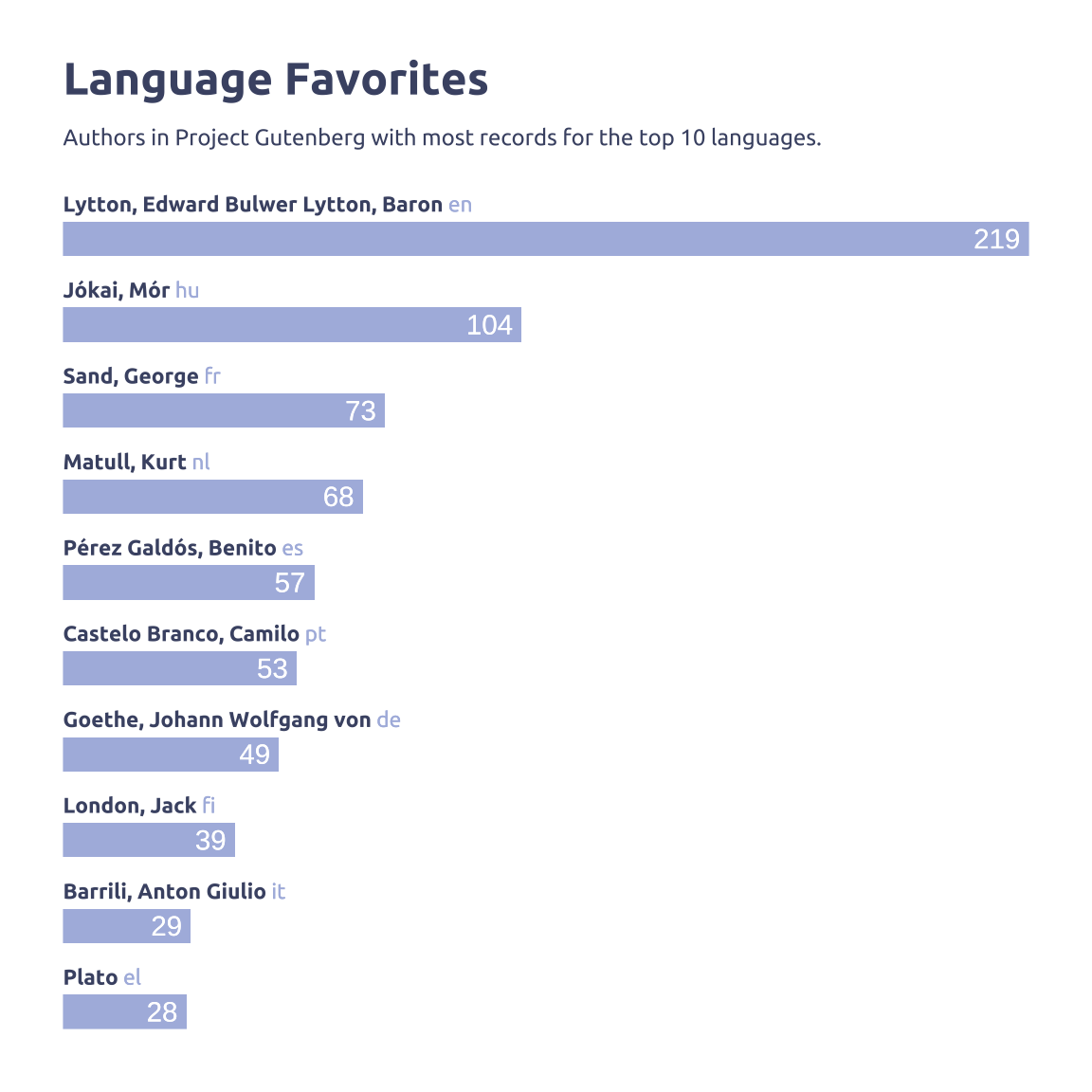
data2plot |>
  ggplot(aes(x = n, y = fct_reorder(author, n))) +
  geom_col(aes(alpha = to_dodge), position = 'dodge', width = 0.8, fill = '#aebae0') +
  geom_text(
    aes(label = comma(n)),
    color = 'white',
    nudge_y = -0.2,
    nudge_x = -2,
    hjust = 1
  ) +
  geom_richtext(
    aes(label = label, alpha = to_dodge),
    x = 0,
    hjust = 0,
    nudge_y = 0.18,
    color = '#495373',
    family = 'Ubuntu',
    size = 3,
    fill = NA,
    label.color = NA, # remove background and outline
    label.padding = grid::unit(rep(0, 4), "pt") # remove padding
  ) +
  scale_alpha_manual(values = c('TRUE' = 0, 'FLASE' = 1)) +
  guides(alpha = 'none') +
  coord_cartesian(expand = FALSE) +
  theme(axis.text.y = element_blank(), axis.text.x = element_blank()) +
  labs(
    x = NULL,
    y = NULL,
    title = 'Language Favorites',
    subtitle = 'Authors in Project Gutenberg with most records for the top 10 languages.')