pacman::p_load(
  tidyverse,
  glue,
  scales,
  showtext,
  ggtext,
  shadowtext,
  maps,
  ggpattern,
  ggrepel,
  patchwork,
  tidylog,
  sf,
  ggblend
)

font_add_google("Ubuntu", "Ubuntu", regular.wt = 400, bold.wt = 700)
showtext_auto()
showtext_opts(dpi = 300)
Tip
About the Data
Note
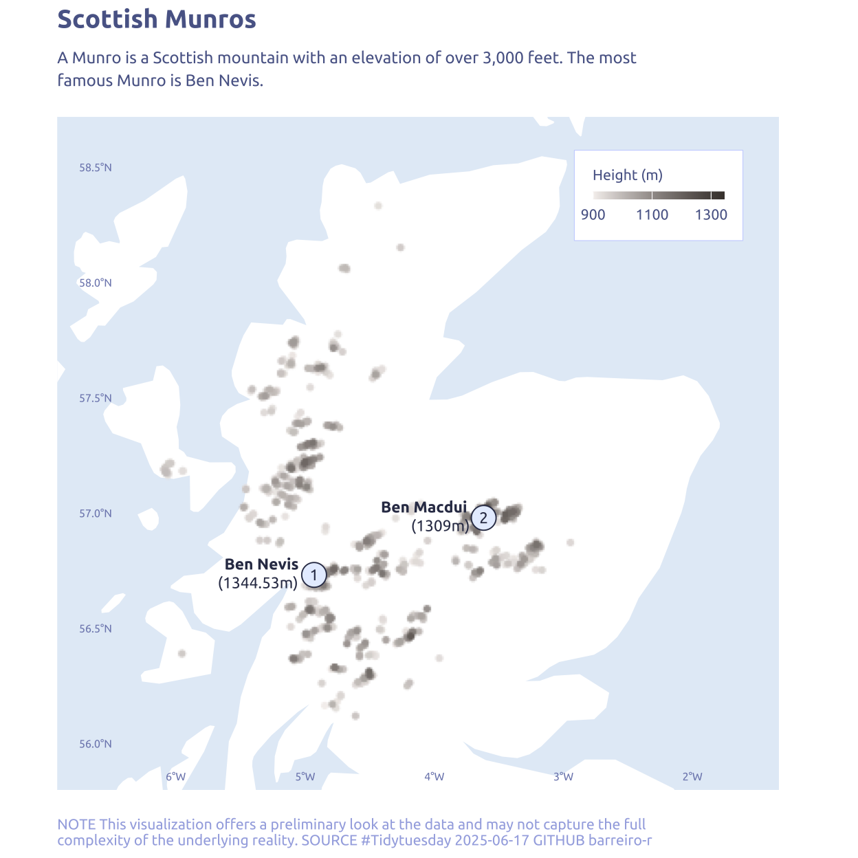
A Munro is a Scottish mountain with an elevation of over 3,000 feet, whereas a Munro Top is a subsidiary summit of a Munro that also exceeds 3,000 feet in height but is not considered a distinct mountain in its own right. The most famous Munro is Ben Nevis.
In 1891, Sir Hugh Munro produced the first list of these hills. However, unlike other classification schemes in Scotland which require a peak to have a prominence of at least 500 feet for inclusion, the Munros lack a rigid set of criteria for inclusion. And so, re-surveying can lead to changes in which peaks are included on the list.
1 Initializing
1.1 Load libraries
1.2 Set theme
cool_gray0 <- "#323955"
cool_gray1 <- "#5a6695"
cool_gray2 <- "#7e89bb"
cool_gray3 <- "#a4aee2"
cool_gray4 <- "#cbd5ff"
cool_gray5 <- "#e7efff"

cool_red0 <- "#A31C44"
cool_red1 <- "#F01B5B"
cool_red2 <- "#F43E75"
cool_red3 <- "#E891AB"
cool_red4 <- "#FAC3D3"
cool_red5 <- "#FCE0E8"

my_colors <- c(
  `Munro` = "#1fc09dff",
  `Munro Top` = "#ffc413ff",
  `Non-Munro` = "#f23a3aff"
)

theme_set(
  theme_minimal() +
    theme(
      # axis.line.x.bottom = element_line(color = 'cool_gray0', linewidth = .3),
      # axis.ticks.x= element_line(color = 'cool_gray0', linewidth = .3),
      # axis.line.y.left = element_line(color = 'cool_gray0', linewidth = .3),
      # axis.ticks.y= element_line(color = 'cool_gray0', linewidth = .3),
      # # panel.grid = element_line(linewidth = .3, color = 'grey90'),
      panel.grid.major = element_blank(),
      panel.grid.minor = element_blank(),
      axis.ticks.length = unit(-0.15, "cm"),
      plot.background = element_blank(),
      # plot.title.position = "plot",
      plot.title = element_text(family = "Ubuntu", size = 14, face = 'bold'),
      plot.caption = element_text(
        size = 8,
        color = cool_gray3,
        margin = margin(20, 0, 0, 0),
        hjust = 0
      ),
      plot.subtitle = element_text(
        size = 9,
        lineheight = 1.15,
        margin = margin(5, 0, 15, 0)
      ),
      axis.title.x = element_markdown(
        family = "Ubuntu",
        hjust = .5,
        size = 8,
        color = cool_gray1
      ),
      axis.title.y = element_markdown(
        family = "Ubuntu",
        hjust = .5,
        size = 8,
        color = cool_gray1
      ),
      axis.text = element_text(
        family = "Ubuntu",
        hjust = .5,
        size = 6,
        color = cool_gray2,
      ),
      axis.text.x = element_text(margin = margin(t = -10)), # Add space above x-axis text
      axis.text.y = element_text(margin = margin(r = -30)), # Add space to the right of y-axis text
      legend.position = "top",
      text = element_text(family = "Ubuntu", color = cool_gray1),
      # plot.margin = margin(25, 25, 25, 25)
    )
)
1.3 Load this week’s data
tuesdata <- tidytuesdayR::tt_load('2025-08-19')2 Quick Exploratory Data Analysis
2.1 Classification over the years
tuesdata$scottish_munros |>
  select(DoBIH_number, `1981`:`2021`) |>
  pivot_longer(-DoBIH_number, names_to = 'year', values_to = 'classification') |>
  mutate(classification = if_else(is.na(classification), 'Non-Munro', classification)) |>
  ggplot(aes(x = year, y = DoBIH_number)) +
  geom_tile(aes(fill = classification)) +
  theme(axis.text.y = element_blank()) +
  scale_fill_manual(values = my_colors)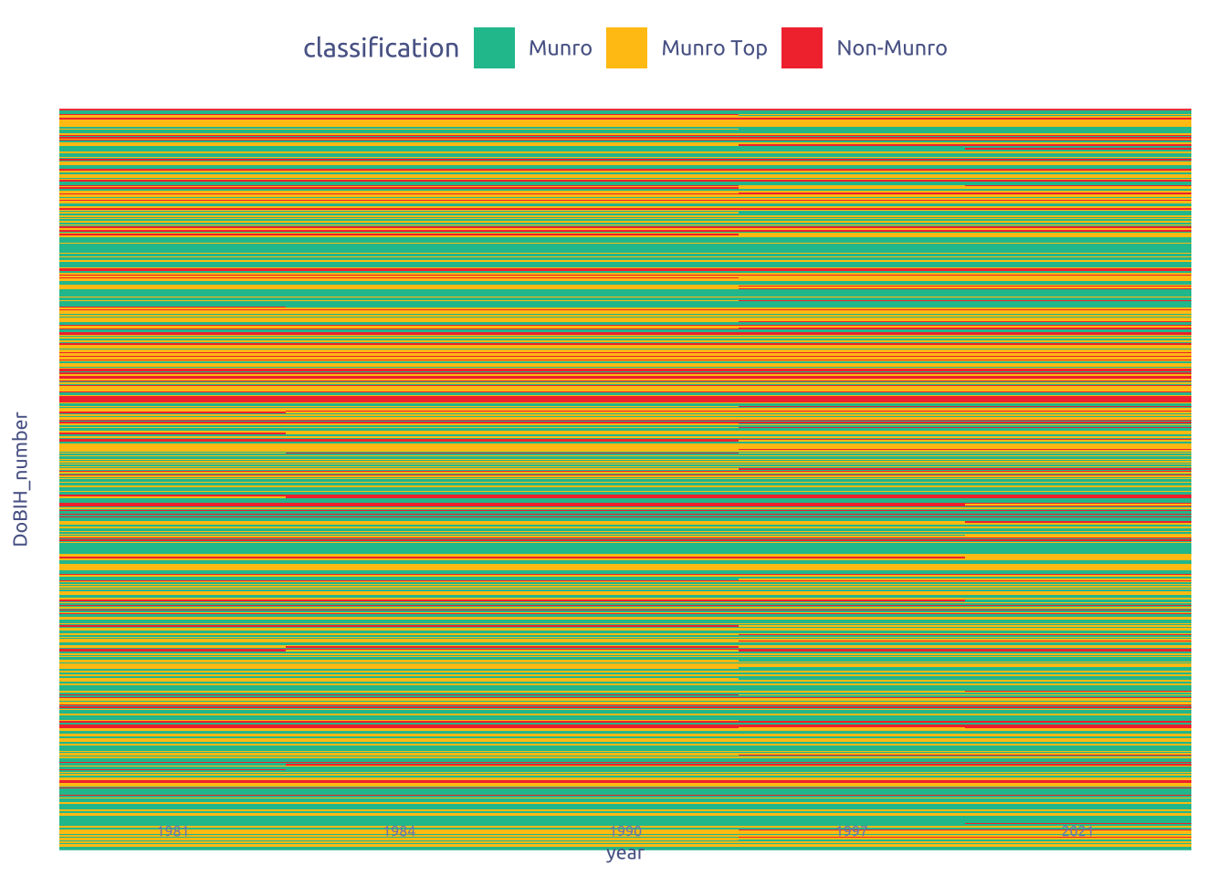
munros_change <-
  tuesdata$scottish_munros |>
  select(DoBIH_number, `1981`:`2021`) |>
  pivot_longer(-DoBIH_number, names_to = 'year', values_to = 'classification') |>
  mutate(classification = if_else(is.na(classification), 'Non-Munro', classification)) |>
  group_by(DoBIH_number) |>
  count(classification) |>
  summarise(n = n()) |>
  filter(n > 1) |>
  pull(DoBIH_number)

tuesdata$scottish_munros |>
  select(DoBIH_number, `1981`:`2021`) |>
  pivot_longer(-DoBIH_number, names_to = 'year', values_to = 'classification') |>
  mutate(classification = if_else(is.na(classification), 'Non-Munro', classification)) |>
  filter(DoBIH_number %in% munros_change) |>
  ggplot(aes(x = year, y = DoBIH_number)) +
  geom_tile(aes(fill = classification)) +
  theme(axis.text.y = element_blank()) +
  scale_fill_manual(values = my_colors)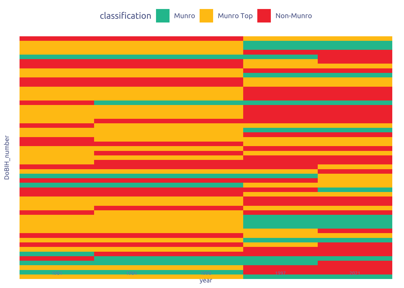
2.2 Geographical distribution
tuesdata$scottish_munros |>
  dplyr::select(xcoord, ycoord, Height_m, `2021`) |>
  ggplot(aes(x = xcoord, y = ycoord, z = Height_m)) +
  stat_summary_hex(
    fun = mean,
    bins = 50
  ) +
  geom_point(
    data = subset(tuesdata$scottish_munros, `2021` == 'Munro') |> dplyr::slice_max(Height_m, n = 3),
    color = "#f60c46ff",
    size = 0.5
  ) +
  scale_fill_gradient(
    low = "#F3F3F3",
    high = "#958277ff") +
  coord_fixed()
3 Transform Data for Plotting
data2plot <-
  tuesdata$scottish_munros |>
  dplyr::select(Name, xcoord, ycoord, Height_m, `2021`) |>
  rename(munro_classification = '2021') |>
  janitor::clean_names() |>
  mutate(munro_classification = if_else(is.na(munro_classification),'Non-Munro', munro_classification))
4 Time to plot!
4.1 Raw chart
tuesdata$scottish_munros |>
  dplyr::select(xcoord, ycoord, Height_m, `2021`) |>
  ggplot(aes(x = xcoord, y = ycoord, z = Height_m)) +
  stat_summary_hex(
    fun = mean,
    bins = 50
  ) +
  geom_point(
    data = subset(tuesdata$scottish_munros, `2021` == 'Munro') |> dplyr::slice_max(Height_m, n = 3),
    color = "#f60c46ff",
    size = 0.5
  ) +
  coord_fixed()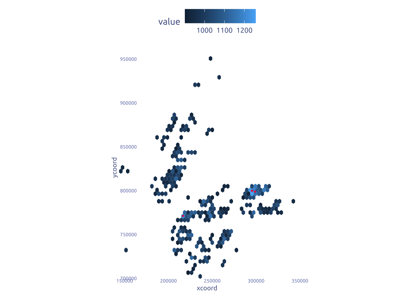
4.2 Final chart
library(sf)
library(ggblend)

data2plot2 <-
  data2plot |>
  filter(!is.na(xcoord)) |>
  st_as_sf(coords = c("xcoord", "ycoord"), crs = "EPSG:27700") |>

  mutate(
    xcoord = st_coordinates(geometry)[, 1],
    ycoord = st_coordinates(geometry)[, 2]
  ) |>

  mutate(name = str_remove(name, " \\[.*"))


xcoord_limits <- c(
  min(data2plot2$xcoord) - 0.25 * min(data2plot2$xcoord),
  max(data2plot2$xcoord) + 0.25 * max(data2plot2$xcoord)
)
ycoord_limits <- c(
  min(data2plot2$ycoord) - 0.03 * min(data2plot2$ycoord),
  max(data2plot2$ycoord) + 0.03 * max(data2plot2$ycoord)
)

data2plot_top1 <-
  data2plot2 |>
  filter(munro_classification == 'Munro') |>
  dplyr::slice_max(height_m, n = 2) |>
  arrange(desc(height_m)) |>
  mutate(rank = row_number())

uk <- rnaturalearth::ne_countries(scale = "medium", returnclass = "sf") |>
  select(name, continent, geometry) |>
  filter(name == "United Kingdom")

ggplot() +
  geom_sf(data = uk, fill = "white", color = NA, size = 0.2) +
  # stat_summary_hex(
  #   data = data2plot2,
  #   aes(
  #     x = st_coordinates(geometry)[, 1],
  #     y = st_coordinates(geometry)[, 2],
  #     z = height_m
  #   ),
  #   fun = mean,
  #   bins = 50
  # ) +
  geom_point(
    data = data2plot2,
    aes(x = xcoord, y = ycoord, color = height_m),
    size = 2,
    stroke = 0)  |> blend("darken") +
  scale_color_gradient(
    limits = c(
      floor(min(data2plot2$height_m)),
      ceiling(max(data2plot2$height_m))
    ),
    n.breaks = 3,
    low = "#f5f1efff",
    high = "#453e3aff"
  ) +
  geom_point(
    data = data2plot_top1,
    aes(x = xcoord, y = ycoord),
    fill = cool_gray5,
    color = cool_gray0,
    size = 6,
    shape = 21
  ) +
  geom_text(
    data = data2plot_top1,
    aes(x = xcoord, y = ycoord, label = rank),
    color = cool_gray0,
    size = 3,
    face = "bold",
    family = "Ubuntu"
  ) +
  ggtext::geom_richtext(
    data = data2plot_top1,
    aes(x = xcoord, y = ycoord, label = glue::glue("**{name}**<br>({height_m}m)")),
    color = cool_gray0,
    size = 3,
    hjust = 1.1,
    family = "Ubuntu",
    fill = NA,
    label.color = NA
  ) +
  coord_sf(xlim = xcoord_limits, ylim = ycoord_limits, crs = "EPSG:27700") +
  theme(
    panel.background = element_rect(fill = "#e3edf7ff", color = NA),
    legend.position = c(.95, .95),
    legend.justification = c(1, 1),
    legend.text = element_text(size = 8),
    legend.title = element_text(size = 8),
    legend.background = element_rect(
      fill = "white",
      color = cool_gray4,
      linewidth = 0.2
    ),
    legend.margin = margin(10, 10, 10, 10),
  ) +
  labs(
    x = NULL,
    y = NULL,
    color = "Height (m)",
    title = "Scottish Munros",
    subtitle =  str_wrap("A Munro is a Scottish mountain with an elevation of over 3,000 feet. The most famous Munro is Ben Nevis.", width = 80),
    caption = str_wrap(
      "NOTE This visualization offers a preliminary look at the data and may not capture the full complexity of the underlying reality. SOURCE #Tidytuesday 2025-06-17 GITHUB barreiro-r",
      width = 100
    )
  ) +
  guides(
    color = guide_colorbar(
      direction = "horizontal",
      barwidth = 5,
      barheight = .3,
      title.position = 'top'
    )
  )