pacman::p_load(
  tidyverse,
  glue,
  scales,
  showtext,
  ggtext,
  shadowtext,
  maps,
  ggpattern,
  ggrepel,
  patchwork,
  tidylog
)

font_add_google("Ubuntu", "Ubuntu", regular.wt = 400, bold.wt = 700)
showtext_auto()
showtext_opts(dpi = 300)
Tip
About the Data
Note
This week we’re exploring 2023 data from the sixth annual release of FrogID data.
FrogID is an Australian frog call identification initiative. The FrogID mobile app allows citizen scientists to record and submit frog calls for museum experts to identify. Since 2017, FrogID data has contributed to over 30 scientific papers exploring frog ecology, taxonomy, and conservation.
Australia is home to a unique and diverse array of frog species found almost nowhere else on Earth, with 257 native species distributed throughout the continent. But Australia’s frogs are in peril – almost one in five species are threatened with extinction due to threats such as climate change, urbanisation, disease, and the spread of invasive species.
1 Initializing
1.1 Load libraries
1.2 Set theme
cool_gray0 <- "#323955"
cool_gray1 <- "#5a6695"
cool_gray2 <- "#7e89bb"
cool_gray3 <- "#a4aee2"
cool_gray4 <- "#cbd5ff"
cool_gray5 <- "#e7efff"

cool_red0 <- "#A31C44"
cool_red1 <- "#F01B5B"
cool_red2 <- "#F43E75"
cool_red3 <- "#E891AB"
cool_red4 <- "#FAC3D3"
cool_red5 <- "#FCE0E8"

theme_set(
  theme_minimal() +
    theme(
      # axis.line.x.bottom = element_line(color = 'cool_gray0', linewidth = .3),
      # axis.ticks.x= element_line(color = 'cool_gray0', linewidth = .3),
      # axis.line.y.left = element_line(color = 'cool_gray0', linewidth = .3),
      # axis.ticks.y= element_line(color = 'cool_gray0', linewidth = .3),
      # # panel.grid = element_line(linewidth = .3, color = 'grey90'),
      panel.grid.major = element_blank(),
      panel.grid.minor = element_blank(),
      axis.ticks.length = unit(-0.15, "cm"),
      plot.background = element_blank(),
      # plot.title.position = "plot",
      plot.title = element_text(family = "Ubuntu", size = 14, face = 'bold'),
      plot.caption = element_text(
        size = 8,
        color = cool_gray3,
        margin = margin(20, 0, 0, 0),
        hjust = 0
      ),
      plot.subtitle = element_text(
        size = 9,
        lineheight = 1.15,
        margin = margin(5, 0, 15, 0)
      ),
      axis.title.x = element_markdown(
        family = "Ubuntu",
        hjust = .5,
        size = 8,
        color = cool_gray1
      ),
      axis.title.y = element_markdown(
        family = "Ubuntu",
        hjust = .5,
        size = 8,
        color = cool_gray1
      ),
      axis.text = element_text(
        family = "Ubuntu",
        hjust = .5,
        size = 8,
        color = cool_gray1
      ),
      legend.position = "top",
      text = element_text(family = "Ubuntu", color = cool_gray1),
      # plot.margin = margin(25, 25, 25, 25)
    )
)
1.3 Load this week’s data
tuesdata <- tidytuesdayR::tt_load('2025-09-02')2 Quick Exploratory Data Analysis
2.1 How many species of frogs were found?
tuesdata$frogID_data |>
  janitor::clean_names() |>
  count(scientific_name, sort = TRUE)
# A tibble: 186 × 2
scientific_name n
<chr> <int>
1 Crinia signifera 33630
2 Limnodynastes peronii 17462
3 Litoria fallax 8572
4 Litoria peronii 8565
5 Limnodynastes tasmaniensis 7372
6 Litoria ewingii 6471
7 Litoria verreauxii 5824
8 Crinia parinsignifera 4339
9 Limnodynastes dumerilii 3289
10 Litoria caerulea 3011
# ℹ 176 more rows2.2 Geografical distribution
tuesdata$frogID_data |>
  janitor::clean_names() |>
  ggplot(aes(x = decimal_longitude, y = decimal_latitude)) +
  geom_point() +
  coord_fixed()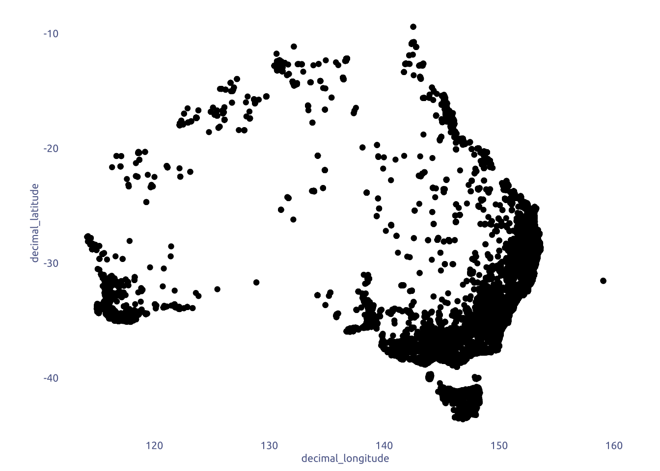
2.2 Geografical distribution by species
most_commom_frogs <- tuesdata$frogID_data |>
  janitor::clean_names() |>
  count(scientific_name, sort = TRUE) |>
  head(10)

tuesdata$frogID_data |>
  janitor::clean_names() |>
  mutate(month = month(event_date)) |>
  mutate(scientific_name = if_else(scientific_name %in% most_commom_frogs$scientific_name, scientific_name, "Other")) |>
  mutate(scientific_name = factor(scientific_name, levels = c(most_commom_frogs$scientific_name, "Other"))) |>
  ggplot(aes(x = decimal_latitude, y = decimal_longitude)) +
  geom_point(aes(color = scientific_name), size = 0.5) +
  facet_grid(month ~ scientific_name) +
  coord_fixed()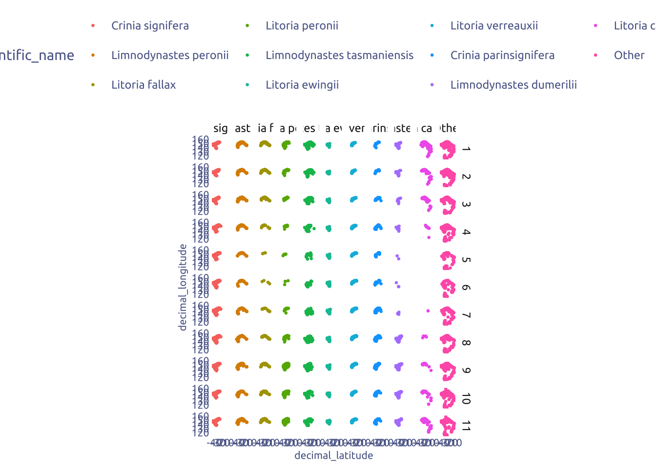
2.2 Geografical distribution by genus
most_commom_frogs_geni <- tuesdata$frogID_data |>
  janitor::clean_names() |>
  mutate(genus = str_remove(scientific_name, ".* ")) |>
  count(genus, sort = TRUE) |>
  head(10)

tuesdata$frogID_data |>
  janitor::clean_names() |>
  mutate(genus = str_remove(scientific_name, ".* ")) |>
  mutate(month = month(event_date)) |>
  mutate(genus = if_else(genus %in% most_commom_frogs_geni$genus, genus, "Other")) |>
  mutate(genus = factor(genus, levels = c(most_commom_frogs_geni$genus, "Other"))) |>
  ggplot(aes(x = decimal_longitude, y = decimal_latitude)) +
  geom_point(aes(color = genus), size = 0.5) +
  facet_grid(month ~ genus) +
  coord_fixed()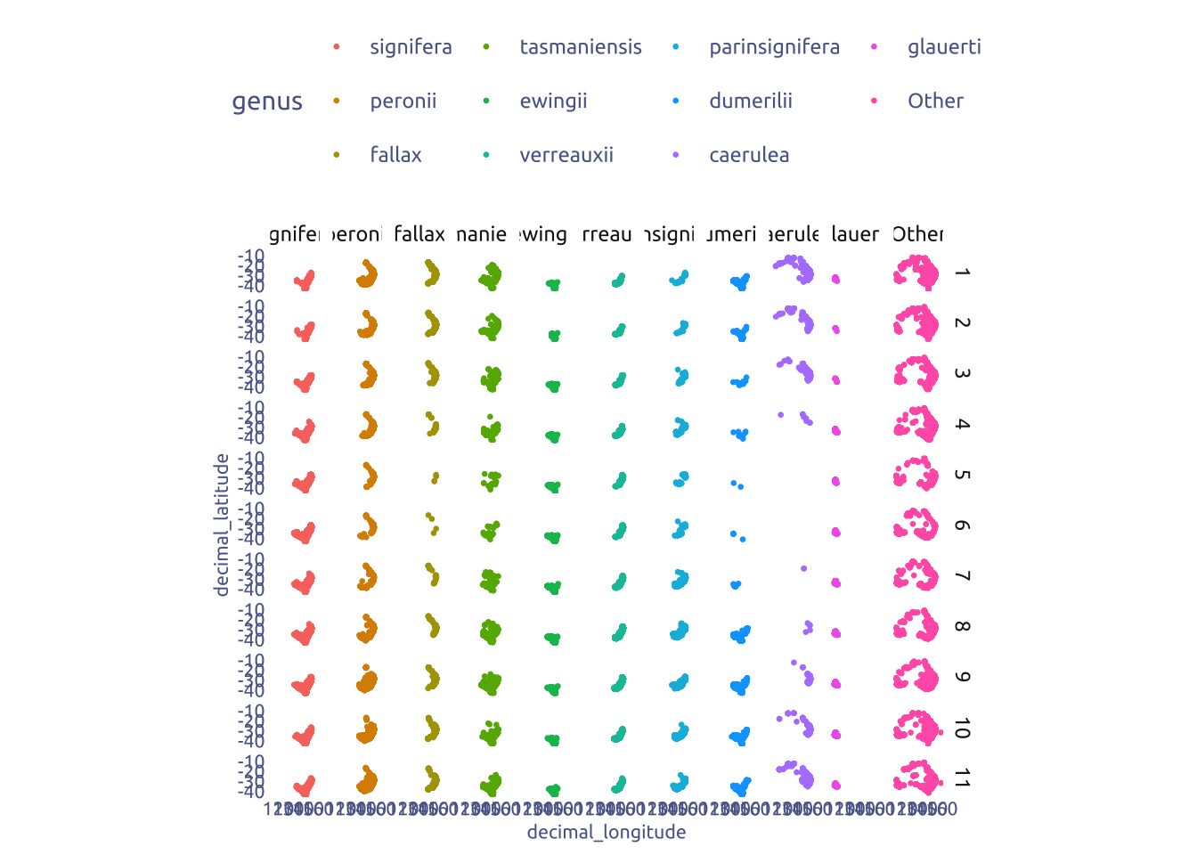
2.2 Geografical distribution by subfamily
most_commom_frogs_subfamilies <- tuesdata$frogID_data |>
  janitor::clean_names() |>
  inner_join(
    tuesdata$frog_names |>
      janitor::clean_names() |>
      select(scientific_name, subfamily, tribe),
    by = "scientific_name"
  ) |>
  mutate(subfamily = str_remove(subfamily, ".* ")) |>
  count(subfamily, sort = TRUE) |>
  head(10)

tuesdata$frogID_data |>
  janitor::clean_names() |>
  inner_join(
    tuesdata$frog_names |>
      janitor::clean_names() |>
      select(scientific_name, subfamily, tribe),
    by = "scientific_name"
  ) |>
  mutate(month = month(event_date)) |>
  ggplot(aes(x = decimal_longitude, y = decimal_latitude)) +
  geom_point(aes(color = subfamily), size = 0.5) +
  facet_wrap(subfamily ~ month, ncol = 11) +
  coord_fixed()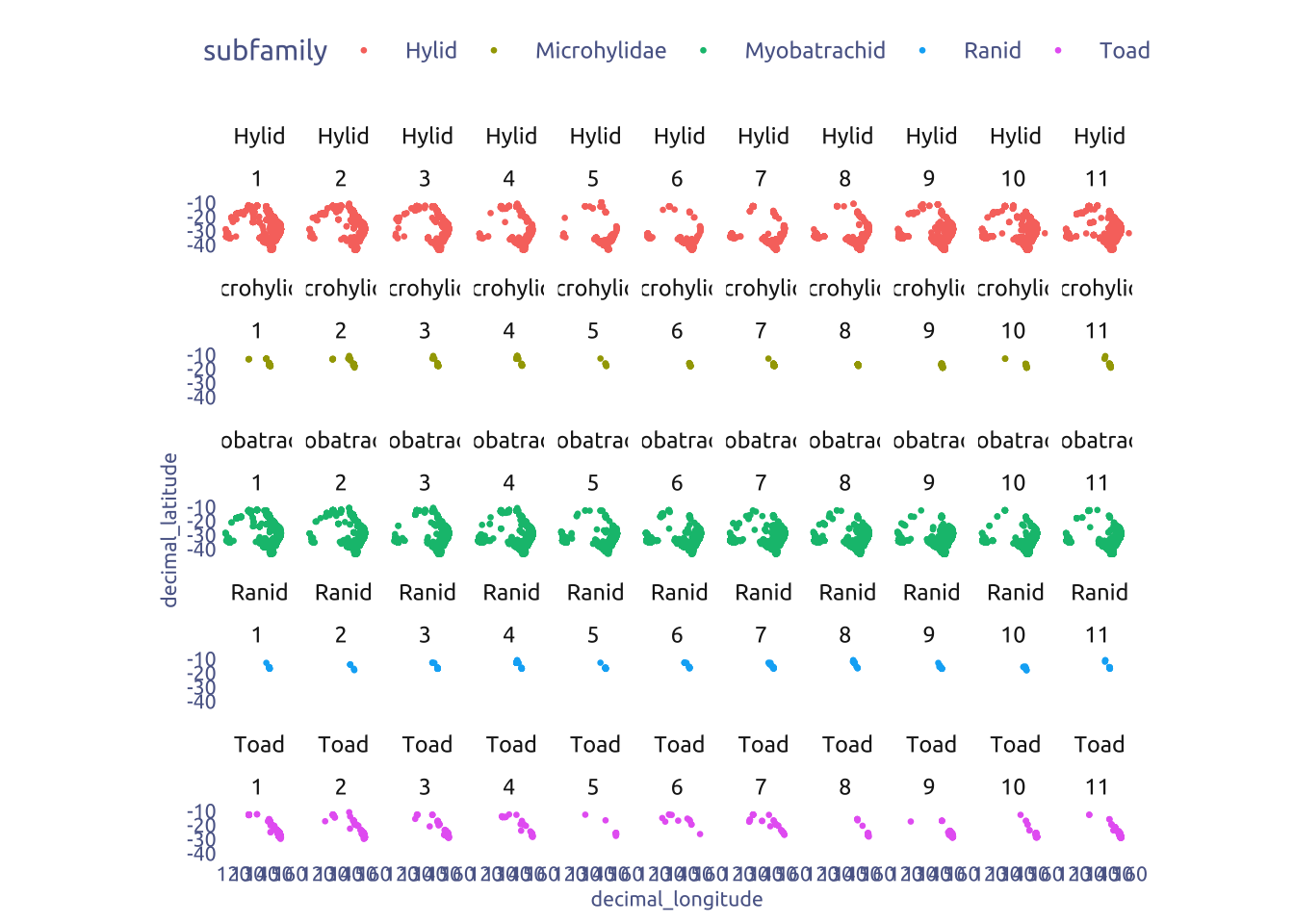
3 Transform Data for Plotting
library(sf)

most_commom_frogs <- tuesdata$frogID_data |>
  janitor::clean_names() |>
  count(scientific_name, sort = TRUE) |>
  head(9) |>
  mutate(scientific_name_rank = str_c(row_number(), ". ", scientific_name))


data2plot <-
  tuesdata$frogID_data |>
  janitor::clean_names() |>
  left_join(
    tuesdata$frog_names |>
      janitor::clean_names() |>
      dplyr::select(scientific_name, subfamily, tribe),
    by = "scientific_name"
  ) |>
  st_as_sf(
    coords = c("decimal_longitude", "decimal_latitude"),
    crs = "EPSG:27700",
    remove = FALSE
  ) |>
  mutate(
    xcoord = st_coordinates(geometry)[, 1],
    ycoord = st_coordinates(geometry)[, 2]
  ) |>
  left_join(most_commom_frogs, by = "scientific_name") |>
  mutate(
    scientific_name_rank = if_else(
      is.na(scientific_name_rank),
      "Other",
      scientific_name_rank
    ),
    scientific_name_rank = factor(
      scientific_name_rank,
      levels = c(most_commom_frogs$scientific_name_rank, "Other")
    )
  )


get_density <- function(x, y, ...) {
  # Calculate the 2D kernel density estimate
  dens <- MASS::kde2d(x, y, ...)

  # Find the intervals for each point in x and y
  ix <- findInterval(x, dens$x)
  iy <- findInterval(y, dens$y)

  # Combine the indices
  ii <- cbind(ix, iy)

  # Return the density value for each point
  return(dens$z[ii])
}

data2plot <- data2plot |>
  group_by(scientific_name_rank) |>
  mutate(
    density_group = get_density(xcoord, ycoord, n = 100)
  ) |>
  mutate(
    z_score_density_group = (density_group - mean(density_group)) / sd(density_group)
  ) |>
  ungroup() |>
  mutate(density = get_density(xcoord, ycoord, n = 100)) |>
  mutate(z_score_density = (density - mean(density)) / sd(density))
4 Time to plot!
4.1 Final chart
au <- rnaturalearth::ne_countries(scale = "large", returnclass = "sf") |>
dplyr::select(name, continent, geometry) |>
filter(name == "Australia")
p_sub <-
ggplot() +
geom_sf(data = au, color = cool_gray3, fill = 'white', linewidth = .2) +
geom_point(
data = data2plot |> filter(scientific_name_rank != "Other"),
aes(x = xcoord, y = ycoord, color = z_score_density_group),
size = 0.3,
show.legend = FALSE
) +
theme(
# panel.background = element_rect(fill = "#e3edf7ff", color = NA)
axis.text = element_blank(),
strip.text = element_text(
color = cool_gray1,
hjust = 0,
family = "Ubuntu",
size = 5
),
) +
coord_sf(xlim = c(112, 155), ylim = c(-45, -10), expand = FALSE) +
facet_wrap(~scientific_name_rank) +
scale_color_gradientn(
colors = (RColorBrewer::brewer.pal(name = "Spectral", n = 8)) |> rev()
) +
labs(x = NULL, y = NULL)
p_main <-
ggplot() +
geom_sf(data = au, color = cool_gray3, fill = 'white', linewidth = .2) +
geom_point(
data = data2plot,
aes(x = xcoord, y = ycoord, color = z_score_density),
size = 0.3,
show.legend = FALSE
) +
theme(
# panel.background = element_rect(fill = "#e3edf7ff", color = NA)
axis.text = element_blank()
) +
coord_sf(xlim = c(112, 155), ylim = c(-45, -10), expand = FALSE) +
scale_color_gradientn(
colors = (RColorBrewer::brewer.pal(name = "Spectral", n = 8)) |> rev()
) +
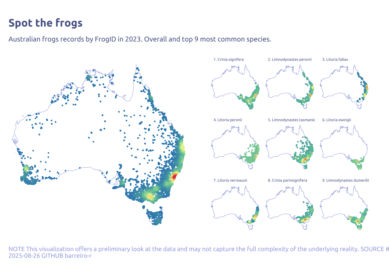
labs(
x = NULL,
y = NULL,
title = "Spot the frogs",
subtitle = "Australian frogs records by FrogID in 2023. Overall and top 9 most common species.",
caption = str_wrap(
"NOTE This visualization offers a preliminary look at the data and may not capture the full complexity of the underlying reality. SOURCE #Tidytuesday 2025-08-26 GITHUB barreiro-r",
width = 150
)
)
p_main + p_sub