pacman::p_load(
  tidyverse,
  glue,
  scales,
  showtext,
  ggtext,
  shadowtext,
  maps,
  ggpattern,
  ggrepel,
  patchwork,
  tidylog
)

font_add_google("Ubuntu", "Ubuntu", regular.wt = 400, bold.wt = 700)
showtext_auto()
showtext_opts(dpi = 300)
Tip
About the Data
Note
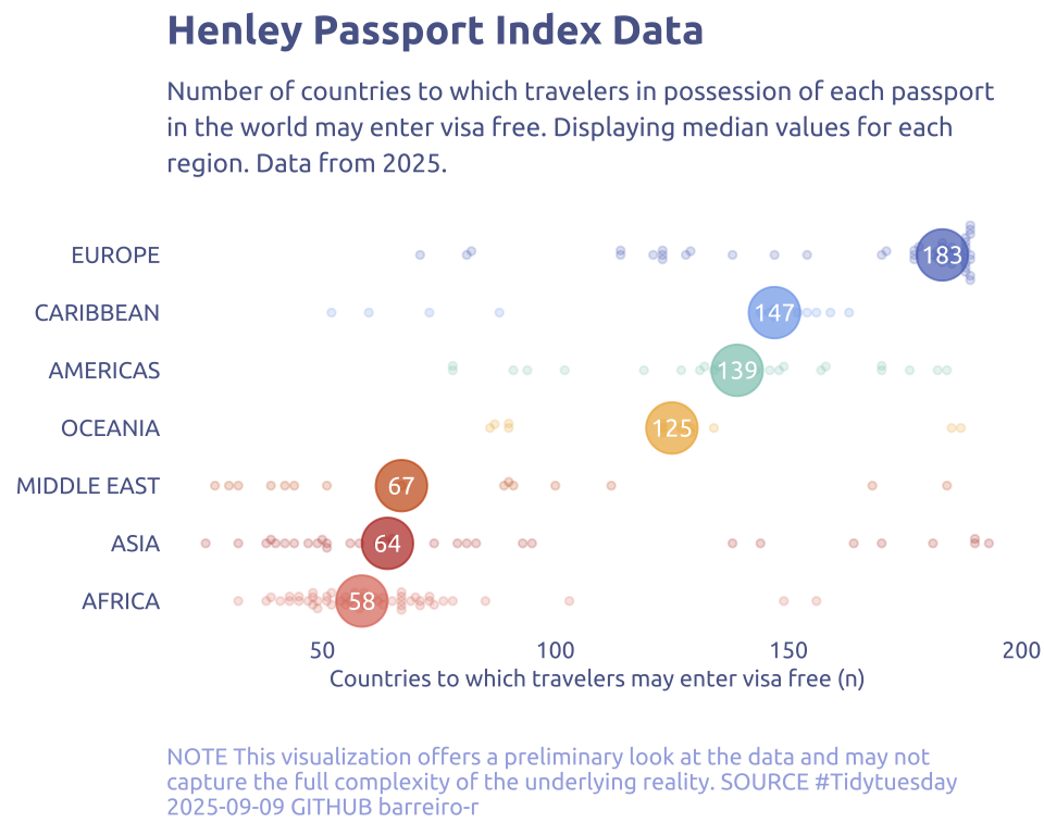
This week we are exploring data from the Henley Passport Index API. The Henley Passport Index is produced by Henley & Partners and captures the number of countries to which travelers in possession of each passport in the world may enter visa free.
1 Initializing
1.1 Load libraries
1.2 Set theme
cool_gray0 <- "#323955"
cool_gray1 <- "#5a6695"
cool_gray2 <- "#7e89bb"
cool_gray3 <- "#a4aee2"
cool_gray4 <- "#cbd5ff"
cool_gray5 <- "#e7efff"

cool_red0 <- "#A31C44"
cool_red1 <- "#F01B5B"
cool_red2 <- "#F43E75"
cool_red3 <- "#E891AB"
cool_red4 <- "#FAC3D3"
cool_red5 <- "#FCE0E8"

theme_set(
  theme_minimal() +
    theme(
      # axis.line.x.bottom = element_line(color = 'cool_gray0', linewidth = .3),
      # axis.ticks.x= element_line(color = 'cool_gray0', linewidth = .3),
      # axis.line.y.left = element_line(color = 'cool_gray0', linewidth = .3),
      # axis.ticks.y= element_line(color = 'cool_gray0', linewidth = .3),
      # # panel.grid = element_line(linewidth = .3, color = 'grey90'),
      panel.grid.major = element_blank(),
      panel.grid.minor = element_blank(),
      axis.ticks.length = unit(-0.15, "cm"),
      plot.background = element_blank(),
      # plot.title.position = "plot",
      plot.title = element_text(family = "Ubuntu", size = 14, face = 'bold'),
      plot.caption = element_text(
        size = 8,
        color = cool_gray3,
        margin = margin(20, 0, 0, 0),
        hjust = 0
      ),
      plot.subtitle = element_text(
        size = 9,
        lineheight = 1.15,
        margin = margin(5, 0, 15, 0)
      ),
      axis.title.x = element_markdown(
        family = "Ubuntu",
        hjust = .5,
        size = 8,
        color = cool_gray1
      ),
      axis.title.y = element_markdown(
        family = "Ubuntu",
        hjust = .5,
        size = 8,
        color = cool_gray1
      ),
      axis.text = element_text(
        family = "Ubuntu",
        hjust = .5,
        size = 8,
        color = cool_gray1
      ),
      legend.position = "top",
      text = element_text(family = "Ubuntu", color = cool_gray1),
      # plot.margin = margin(25, 25, 25, 25)
    )
)
1.3 Load this week’s data
tuesdata <- tidytuesdayR::tt_load('2025-09-09')2 Quick Exploratory Data Analysis
2.1 Density: Countries x Years
tuesdata$rank_by_year |>
  count(year, sort = TRUE)
# A tibble: 20 × 2
year n
<dbl> <int>
1 2010 199
2 2011 199
3 2012 199
4 2013 199
5 2014 199
6 2015 199
7 2016 199
8 2017 199
9 2018 199
10 2019 199
11 2020 199
12 2021 199
13 2022 199
14 2023 199
15 2024 199
16 2025 199
17 2008 198
18 2009 198
19 2006 185
20 2007 185Wow, very complete data. Is this the real world?
tuesdata$rank_by_year |>
  filter(year == 2021) |>
  slice_max(visa_free_count, n = 10)
# A tibble: 10 × 6
code country region rank visa_free_count year
<chr> <chr> <chr> <dbl> <dbl> <dbl>
1 JP Japan ASIA 1 192 2021
2 SG Singapore ASIA 1 192 2021
3 DE Germany EUROPE 2 190 2021
4 KR South Korea ASIA 2 190 2021
5 FI Finland EUROPE 3 189 2021
6 IT Italy EUROPE 3 189 2021
7 LU Luxembourg EUROPE 3 189 2021
8 ES Spain EUROPE 3 189 2021
9 AT Austria EUROPE 4 188 2021
10 DK Denmark EUROPE 4 188 2021tuesdata$rank_by_year |>
filter(year == 2021) |>
slice_min(visa_free_count, n = 10)# A tibble: 12 × 6
code country region rank visa_free_count year
<chr> <chr> <chr> <dbl> <dbl> <dbl>
1 AF Afghanistan ASIA 116 26 2021
2 IQ Iraq MIDDLE EAST 115 28 2021
3 SY Syria MIDDLE EAST 114 29 2021
4 PK Pakistan ASIA 113 31 2021
5 YE Yemen MIDDLE EAST 112 33 2021
6 SO Somalia AFRICA 111 34 2021
7 NP Nepal ASIA 110 37 2021
8 PS Palestinian Territory MIDDLE EAST 110 37 2021
9 KP North Korea ASIA 109 39 2021
10 BD Bangladesh ASIA 108 40 2021
11 XK Kosovo EUROPE 108 40 2021
12 LY Libya AFRICA 108 40 20213 Transform Data for Plotting
data2plot <-
  tuesdata$rank_by_year |>
  filter(year == 2025)

data2plot_summary <-
  tuesdata$rank_by_year |>
  filter(year == 2025) |>
  group_by(region) |>
  summarize(
    min_vfc = min(visa_free_count),
    max_vfc = max(visa_free_count),
    mean_vfc = mean(visa_free_count),
    median_vfc = median(visa_free_count),
    sd_vfc = sd(visa_free_count),
    iqr_vfc = IQR(visa_free_count),
  ) |>
  ungroup()
4 Time to plot!
4.1 Raw chart
ggplot(data2plot_summary, aes(x = region, y = median_vfc)) +
  geom_col() +
  theme_grey()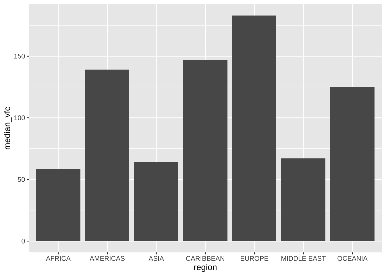
4.2 Final chart
data2plot_summary |>
  mutate(region = fct_reorder(region, median_vfc)) |>
  ggplot(aes(x = median_vfc, y = region)) +
  ggbeeswarm::geom_beeswarm(
    data = data2plot,
    aes(x = visa_free_count, y = region, color = region),
    size = 1,
    alpha = .2,
    cex = 1.1
  ) +
  #border
  geom_point(aes(color = region), size = 8, alpha = .7) +
  geom_text(
    aes(label = floor(median_vfc)),
    color = 'white',
    family = 'Ubuntu',
    size = 3,
    hjust = 0.5,
    vjust = 0.5
  ) +
  guides(color = 'none') +
  scale_color_manual(values = MetBrewer::met.brewer("Nizami")) +
  labs(
    x = "Countries to which travelers may enter visa free (n)",
    y = NULL,
    title = "Henley Passport Index Data",
    subtitle = str_wrap(
      "Number of countries to which travelers in possession of each passport in the world may enter visa free. Displaying median values for each region. Data from 2025.",
      width = 70
    ),
    caption = str_wrap(
      "NOTE This visualization offers a preliminary look at the data and may not capture the full complexity of the underlying reality. SOURCE #Tidytuesday 2025-09-09 GITHUB barreiro-r",
      width = 80,
    )
  )