pacman::p_load(
  tidyverse,
  glue,
  scales,
  showtext,
  ggtext,
  shadowtext,
  maps,
  ggpattern,
  ggrepel,
  patchwork,
  tidylog
)

font_add_google("Ubuntu", "Ubuntu", regular.wt = 400, bold.wt = 700)
showtext_auto()
showtext_opts(dpi = 300)
Tip
About the Data
Note
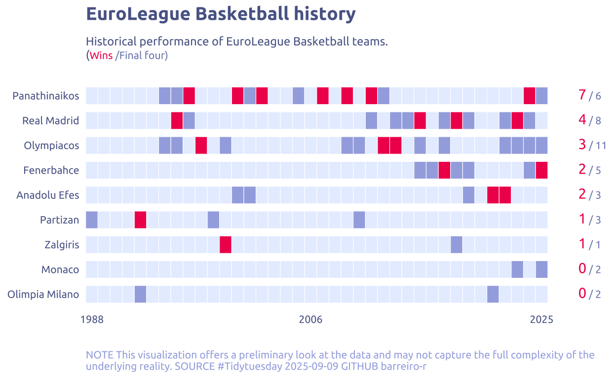
This week we’re exploring EuroLeague Basketball, the premier men’s club basketball competition in Europe.
The dataset contains information on EuroLeague teams, including their country, home city, arena, seating capacity, and historical performance (Final Four appearances and titles won).
The dataset is curated from publicly available sources such as Wikipedia and official EuroLeague records, and was packaged in the EuroleagueBasketball R package, with documentation available at natanast.github.io/EuroleagueBasketball.
“The EuroLeague is the top-tier European professional basketball club competition, widely regarded as the most prestigious competition in European basketball.” — EuroLeague
1 Initializing
1.1 Load libraries
1.2 Set theme
cool_gray0 <- "#323955"
cool_gray1 <- "#5a6695"
cool_gray2 <- "#7e89bb"
cool_gray3 <- "#a4aee2"
cool_gray4 <- "#cbd5ff"
cool_gray5 <- "#e7efff"

cool_red0 <- "#A31C44"
cool_red1 <- "#F01B5B"
cool_red2 <- "#F43E75"
cool_red3 <- "#E891AB"
cool_red4 <- "#FAC3D3"
cool_red5 <- "#FCE0E8"

theme_set(
  theme_minimal() +
    theme(
      # axis.line.x.bottom = element_line(color = 'cool_gray0', linewidth = .3),
      # axis.ticks.x= element_line(color = 'cool_gray0', linewidth = .3),
      # axis.line.y.left = element_line(color = 'cool_gray0', linewidth = .3),
      # axis.ticks.y= element_line(color = 'cool_gray0', linewidth = .3),
      # # panel.grid = element_line(linewidth = .3, color = 'grey90'),
      panel.grid.major = element_blank(),
      panel.grid.minor = element_blank(),
      axis.ticks.length = unit(-0.15, "cm"),
      plot.background = element_blank(),
      # plot.title.position = "plot",
      plot.title = element_text(family = "Ubuntu", size = 14, face = 'bold'),
      plot.caption = element_text(
        size = 8,
        color = cool_gray3,
        margin = margin(20, 0, 0, 0),
        hjust = 0
      ),
      plot.subtitle = element_markdown(
        size = 9,
        lineheight = 1.15,
        margin = margin(5, 0, 15, 0)
      ),
      axis.title.x = element_markdown(
        family = "Ubuntu",
        hjust = .5,
        size = 8,
        color = cool_gray1
      ),
      axis.title.y = element_markdown(
        family = "Ubuntu",
        hjust = .5,
        size = 8,
        color = cool_gray1
      ),
      axis.text = element_text(
        family = "Ubuntu",
        hjust = .5,
        size = 8,
        color = cool_gray1
      ),
      legend.position = "top",
      text = element_text(family = "Ubuntu", color = cool_gray1),
      # plot.margin = margin(25, 25, 25, 25)
    )
)
1.3 Load this week’s data
tuesdata <- tidytuesdayR::tt_load('2025-10-07')2 Quick Exploratory Data Analysis
2.1 Arena Capacity
tuesdata$euroleague_basketball |>
  janitor::clean_names() |>
  select(team,capacity, titles_won) |>
  mutate(capacity = str_remove_all(capacity, ',')) |>
  mutate(capacity = str_split(capacity, " ")) |>
  unnest(capacity) |>
  mutate(capacity = as.numeric(capacity)) |>
  group_by(team) |> filter(capacity == max(capacity)) |> ungroup() |>
  mutate(team = fct_reorder(team, capacity, .fun = max)) |>
  ggplot(aes(y = team, x = capacity)) +
  geom_col(fill = cool_gray1) +
  labs(title = "Arena Capacity", x = "Capacity", y = NULL) +
scale_x_continuous(label = scales::comma, expand = c(0,0)) 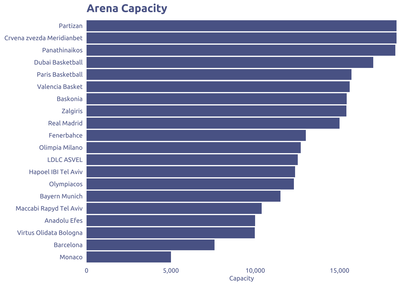
2.2 Titles Won
tuesdata$euroleague_basketball |>
  janitor::clean_names() |>
  select(team,capacity, titles_won) |>
  mutate(capacity = str_remove_all(capacity, ',')) |>
  mutate(capacity = str_split(capacity, " ")) |>
  unnest(capacity) |>
  mutate(capacity = as.numeric(capacity)) |>
  group_by(team) |> filter(capacity == max(capacity)) |> ungroup() |>
  mutate(team = fct_reorder(team, titles_won, .fun = max)) |>
  ggplot(aes(y = team, x = titles_won)) +
  geom_col(fill = cool_gray1) +
  labs(title = "Titles Won", x = "Titles Won", y = NULL) +
scale_x_continuous(label = scales::comma, expand = c(0,0)) 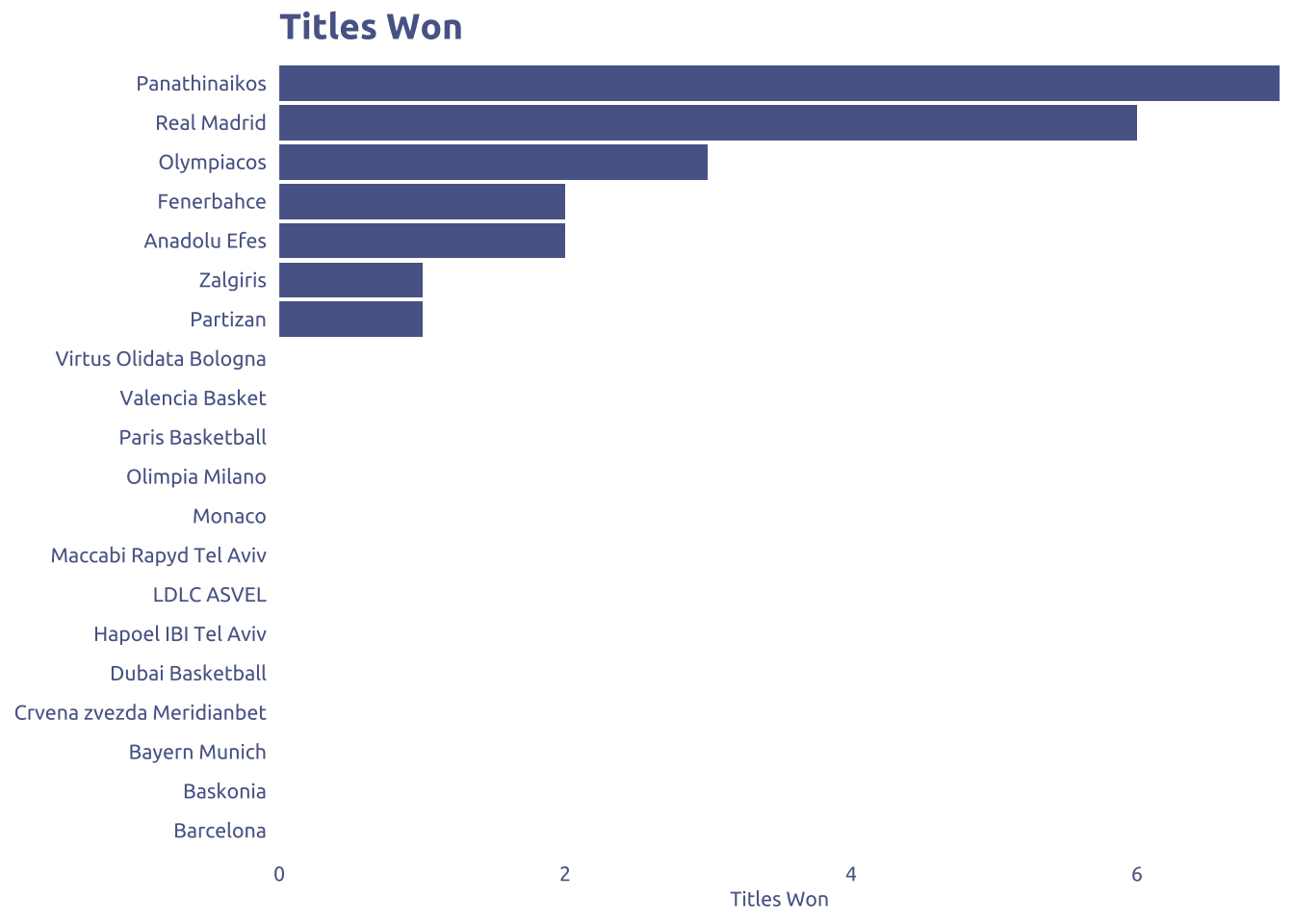
2.3 Country
tuesdata$euroleague_basketball |>
  janitor::clean_names() |>
  count(country) |>
  mutate(country = fct_reorder(country, n)) |>
  ggplot(aes(y = country, x = n)) +
  geom_col(fill = cool_gray1) +
  labs(title = "Teams by Country", x = "Teams (n)", y = NULL) +
scale_x_continuous(label = scales::comma, expand = c(0,0)) 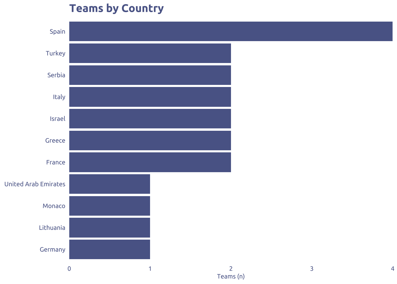
3 Transform Data for Plotting
years <-
  tuesdata$euroleague_basketball |>
  janitor::clean_names() |>
  # select(team, years_of_final_four_appearances, years_of_titles_won) |>
  transmute(years = str_split(years_of_final_four_appearances, ", ")) |>
  unnest(years) |>
  na.omit() |>
  filter(years %in% c(max(years), min(years))) |>
  distinct() |>
  mutate(years = as.numeric(years)) |>
  arrange(years) |>
  mutate(year_categ = c('first', 'last')) |>
  pull(years, name = year_categ)

years <- seq(years[['first']], years[['last']])

teams <-
  tuesdata$euroleague_basketball |>
  janitor::clean_names() |>
  distinct(team) |>
  pull()

year_in_final_four <-
  tuesdata$euroleague_basketball |>
  janitor::clean_names() |>
  select(team, years_of_final_four_appearances, years_of_titles_won) |>
  transmute(team, years = str_split(years_of_final_four_appearances, ", ")) |>
  unnest(years) |>
  filter(!is.na(years)) |>
  mutate(years = as.numeric(years)) |>
  rename(year = "years") |>
  mutate(status = "final_four")

year_won <-
  tuesdata$euroleague_basketball |>
  janitor::clean_names() |>
  select(team, years_of_titles_won) |>
  transmute(team, years = str_split(years_of_titles_won, ", ")) |>
  unnest(years) |>
  filter(!is.na(years)) |>
  filter(years != "None") |>
  mutate(years = as.numeric(years)) |>
  rename(year = "years") |>
  mutate(status = "win")

data2plot <-
  expand_grid(team = teams, year = years) |>
  left_join(year_won, by = c("year", "team")) |>
  rows_patch(year_in_final_four, by = c("year", "team")) |>
  mutate(
    status_height = case_when(
      is.na(status) ~ 0,
      status == "final_four" ~ 1,
      status == "win" ~ 2,
      TRUE ~ NA
    )) |>
    group_by(team) |>
    filter(sum(status_height) > 0) |>
    ungroup()


team_order <-
  data2plot |>
  count(team,status, sort = TRUE) |> filter(!is.na(status)) |>
  pivot_wider(values_from = 'n', names_from = 'status') |>
  arrange(desc(win), desc(final_four)) |>
  pull(team)


data2plot <-
  data2plot |>
  mutate(team = factor(team, levels = team_order))
4 Time to plot!
4.1 Raw chart
data2plot |>
  ggplot(aes(x = year, y = team)) +
  geom_tile(aes(fill = status), color = 'white') +
  theme_gray()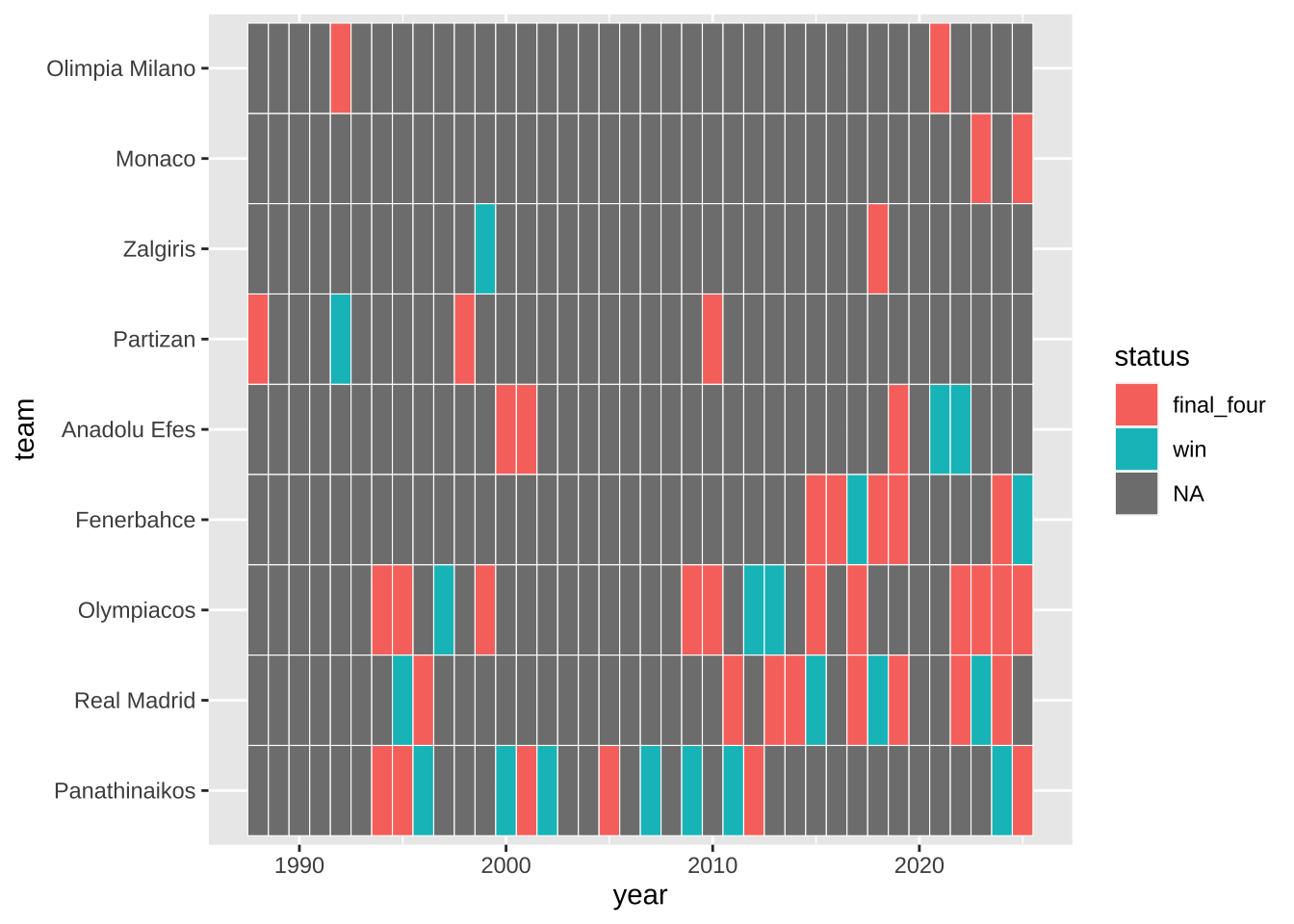
4.2 Final chart
p1 <-
  data2plot |>
  mutate(status = if_else(is.na(status), "none", status)) |>
  mutate(team = factor(team, levels = rev(team_order))) |>
  ggplot(aes(x = year, y = team)) +
  geom_tile(
    aes(fill = status),
    color = 'white',
    show.legend = FALSE,
    height = .7
  ) +
  scale_fill_manual(
    values = c(win = cool_red1, final_four = cool_gray3, none = cool_gray5)
  ) +
  scale_x_continuous(
    expand = c(0, 0),
    breaks = seq(min(years), max(years), length.out = 3) |> round()
  ) +
  labs(
    x = NULL,
    y = NULL,
    x = "Average Age (y)",
    y = NULL,
    title = "EuroLeague Basketball history",
    subtitle = str_wrap(
      glue("Historical performance of EuroLeague Basketball teams.<br>(<span style='font-size:8pt; color:{cool_red1}'>Wins</span><span style='font-size:8pt; color:{cool_gray2}'> /Final four)</span>"),
      width = 100,
    ),
    caption = str_wrap(
      "NOTE This visualization offers a preliminary look at the data and may not capture the full complexity of the underlying reality. SOURCE #Tidytuesday 2025-09-09 GITHUB barreiro-r",
      width = 110,
    )
  ) +
  theme(plot.margin = margin(0, 0, 0, 0))

p2 <-
  data2plot |>
  mutate(status = if_else(is.na(status), "none", status)) |>
  mutate(team = factor(team, levels = rev(team_order))) |>
  count(status, team) |>
  filter(!is.na(status)) |>
  pivot_wider(names_from = status, values_from = n, values_fill = 0) |>
  mutate(
    label = glue(
      "<span style='font-size:11pt; color:{cool_red1}'>{win}</span><span style='font-size:8pt; color:{cool_gray2}'> / {final_four}</span>"
    )
  ) |>
  ggplot(aes(x = 1, y = team)) +
  ggtext::geom_richtext(
    aes(label = label, x = 1),
    fill = NA,
    label.color = NA,
    label.padding = grid::unit(rep(0, 4), "pt"),
    family = "Ubuntu",
    hjust = 0
  ) +
  theme_void() +
  theme(plot.margin = margin(0, 0, 0, 0))

p1 + p2 + patchwork::plot_layout(widths = c(5.3, 0.7), axes = "collect_y")