pacman::p_load(
  tidyverse,
  glue,
  scales,
  showtext,
  ggtext,
  shadowtext,
  maps,
  ggpattern,
  ggrepel,
  patchwork,
  tidylog,
  tidytext,
  textdata,
  syuzhet
)

font_add_google("Ubuntu", "Ubuntu", regular.wt = 400, bold.wt = 700)
showtext_auto()
showtext_opts(dpi = 300)
Tip
About the Data
Note
This week we’re exploring the complete line-by-line text of the Sherlock Holmes stories and novels, made available through the {sherlock} R package by Emil Hvitfeldt. The dataset includes the full collection of Holmes texts, organized by book and line number, and is ideal for stylometry, sentiment analysis, and literary exploration.
“The name is Sherlock Holmes and the address is 221B Baker Street.” Holmes is a consulting detective known for his keen observation, logical reasoning, and use of forensic science to solve complex cases. Created by Sir Arthur Conan Doyle, Holmes has become one of the most famous fictional detectives in literature.
1 Initializing
1.1 Load libraries
1.2 Set theme
cool_gray0 <- "#323955"
cool_gray1 <- "#5a6695"
cool_gray2 <- "#7e89bb"
cool_gray3 <- "#a4aee2"
cool_gray4 <- "#cbd5ff"
cool_gray5 <- "#e7efff"

cool_red0 <- "#A31C44"
cool_red1 <- "#F01B5B"
cool_red2 <- "#F43E75"
cool_red3 <- "#E891AB"
cool_red4 <- "#FAC3D3"
cool_red5 <- "#FCE0E8"

theme_set(
  theme_minimal() +
    theme(
      # axis.line.x.bottom = element_line(color = 'cool_gray0', linewidth = .3),
      # axis.ticks.x= element_line(color = 'cool_gray0', linewidth = .3),
      # axis.line.y.left = element_line(color = 'cool_gray0', linewidth = .3),
      # axis.ticks.y= element_line(color = 'cool_gray0', linewidth = .3),
      # # panel.grid = element_line(linewidth = .3, color = 'grey90'),
      panel.grid.major = element_blank(),
      panel.grid.minor = element_blank(),
      axis.ticks.length = unit(-0.15, "cm"),
      plot.background = element_blank(),
      # plot.title.position = "plot",
      plot.title = element_text(family = "Ubuntu", size = 14, face = 'bold'),
      plot.caption = element_text(
        size = 8,
        color = cool_gray3,
        margin = margin(20, 0, 0, 0),
        hjust = 0
      ),
      plot.subtitle = element_markdown(
        size = 9,
        lineheight = 1.15,
        margin = margin(5, 0, 15, 0)
      ),
      axis.title.x = element_markdown(
        family = "Ubuntu",
        hjust = .5,
        size = 8,
        color = cool_gray1
      ),
      axis.title.y = element_markdown(
        family = "Ubuntu",
        hjust = .5,
        size = 8,
        color = cool_gray1
      ),
      axis.text = element_text(
        family = "Ubuntu",
        hjust = .5,
        size = 8,
        color = cool_gray1
      ),
      legend.position = "top",
      text = element_text(family = "Ubuntu", color = cool_gray1),
      plot.margin = margin(25, 25, 25, 25)
    )
)
1.3 Load this week’s data
tuesdata <- tidytuesdayR::tt_load('2025-11-18')2 Quick Exploratory Data Analysis
2.1 Book Length
tuesdata$holmes |>
  count(book) |>
  mutate(book = fct_reorder(book, n)) |>
  ggplot(aes(x = n, y = book)) +
  geom_col()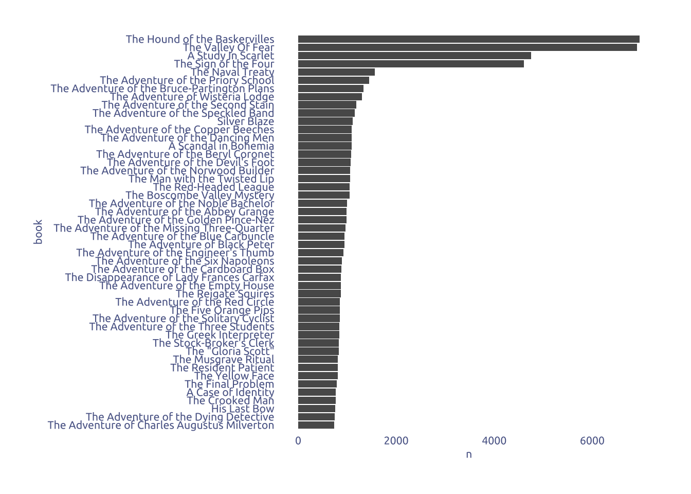
3 Transform Data for Plotting
library(tidytext)

# sherlock_tokens <- tuesdata$holmes |>
#   unnest_tokens(word, text) |>
#   anti_join(stop_words, by = "word")

# nrc_lexicon <- get_sentiments("nrc")

# sherlock_nrc <- sherlock_tokens |>
#   inner_join(nrc_lexicon, by = "word") |>
#   filter(!sentiment %in% c("positive", "negative")) |>
#   group_by(book) |>
#   mutate(word_order = row_number()) |>
#   # mutate(chunk = word_order %/% 20) |>
#   mutate(chunk = ntile(word_order, 100)) |>
#   ungroup() |>
#   count(book, sentiment, chunk) |>
#   group_by(book, chunk) |>
#   slice_max(order_by = n, n = 1, with_ties = FALSE) |>
#   ungroup()

# data2plot <-
#   sherlock_nrc |>
#   select(book, sentiment, chunk)

# data2plot_wide <-
#   data2plot |>
#   mutate(chunk = str_c("chunk", chunk)) |>
#   pivot_wider(values_from = sentiment, names_from = 'chunk') |>
#   column_to_rownames(var = "book") |>
#   mutate(across(everything(), as.factor))

# gower_dist <- cluster::daisy(data2plot_wide, metric = "gower")
# hc_books <- hclust(gower_dist, method = "complete")

# order <- hc_books$labels[hc_books$order]

# data2plot <-
#   mutate(data2plot, book = factor(book, levels = order))

scores <- tuesdata$holmes$text |> get_sentiment()

data2plot <- tuesdata$holmes |>
  mutate(sentiment = scores) |>
  group_by(book) |>
  mutate(chunk = ntile(line_num, 100)) |>
  group_by(book, chunk) |>
  summarise(sentiment = mean(sentiment, na.rm = TRUE)) |>
  ungroup()

# Select the three top and bottom books by mean sentiment
top3 <-
  data2plot |>
  group_by(book) |>
  summarise(sentiment = mean(sentiment, na.rm = TRUE)) |>
  ungroup() |>
  slice_max(order_by = sentiment, n = 3, with_ties = FALSE) |>
  pull(book)

bottom3 <-
  data2plot |>
  group_by(book) |>
  summarise(sentiment = mean(sentiment, na.rm = TRUE)) |>
  ungroup() |>
  slice_min(order_by = sentiment, n = 3, with_ties = FALSE) |>
  pull(book)

data2plot_wide <-
  data2plot |>
  filter(book %in% c(top3, bottom3)) |>
  mutate(chunk = str_c("chunk", chunk)) |>
  pivot_wider(values_from = sentiment, names_from = 'chunk') |>
  column_to_rownames(var = "book") |>
  mutate(across(everything(), as.factor))

# hc_books <- hclust(dist(data2plot_wide), method = "complete")
# order <- hc_books$labels[hc_books$order]

# data2plot <- data2plot |>
#   filter(book %in% c(top3, bottom3)) |>
#   mutate(book = factor(book, levels = order))

data2plot <- data2plot |>
  filter(book %in% c(top3, bottom3)) |>
  mutate(book = factor(book, levels = c(top3,bottom3)))
4 Time to plot!
4.1 Raw chart
data2plot |>
  ggplot(aes(x = chunk, y = sentiment)) +
  geom_line() +
  facet_wrap(~ book, ncol = 2) +
  theme_gray()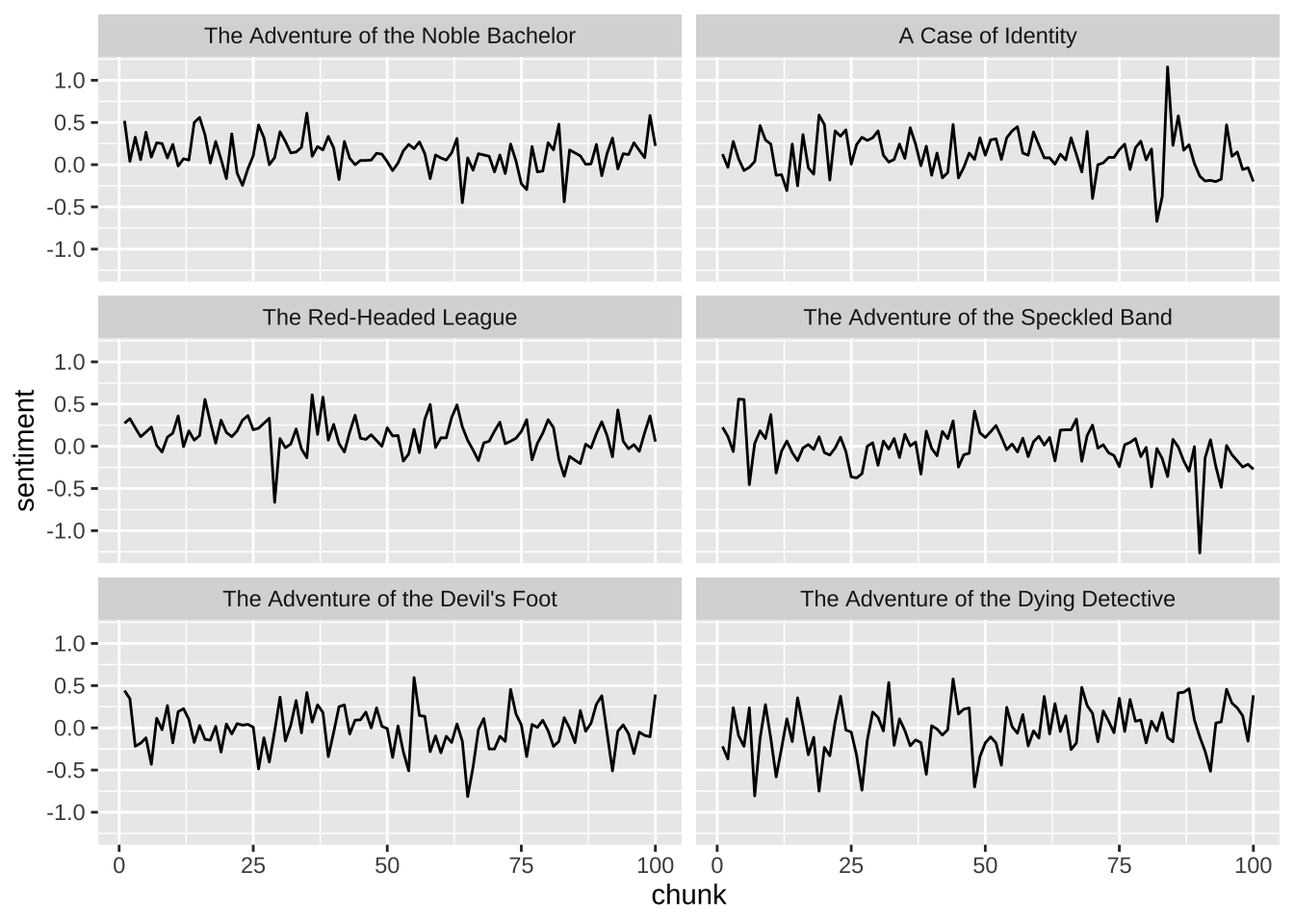
4.2 Final chart
data2plot |>
ggplot(aes(x = chunk, y = sentiment)) +
annotate(
geom = "segment",
y = 0,
yend = 0,
x = -Inf,
xend = Inf,
color = cool_gray5,
linewidth = 0.5,
) +
ggforce::geom_link2(aes(color = sentiment)) +
geom_point(
data = data2plot |>
group_by(book) |>
slice_max(sentiment, n = 1, with_ties = FALSE),
aes(color = sentiment),
size = .7
) +
geom_point(
data = data2plot |>
group_by(book) |>
slice_min(sentiment, n = 1, with_ties = FALSE),
aes(color = sentiment),
size = .7
) +
facet_wrap(~book, ncol = 2) +
theme(
axis.text = element_blank(),
axis.title.x = element_blank(),
axis.title.y = element_blank(),
strip.text.x = element_text(
hjust = 0,
color = cool_gray1,
size = 7,
family = "Ubuntu"
),
legend.position = "bottom",
legend.text = element_text(
size = 7,
),
legend.ticks = element_blank()
) +
scale_color_gradientn(
limits = c(
-1 * max(abs(data2plot$sentiment)),
1 * max(abs(data2plot$sentiment))
),
# colors = MetBrewer::met.brewer("Troy"),
colors = rev(c(
cool_gray0,
cool_gray1,
cool_gray2,
cool_red2,
cool_red1,
cool_red0
)),
breaks = c(-0.7, 0.7),
labels = c("Negative", "Positive")
) +
guides(
color = guide_colorbar(
barwidth = 9,
barheight = .3
)
) +
labs(
color = NULL,
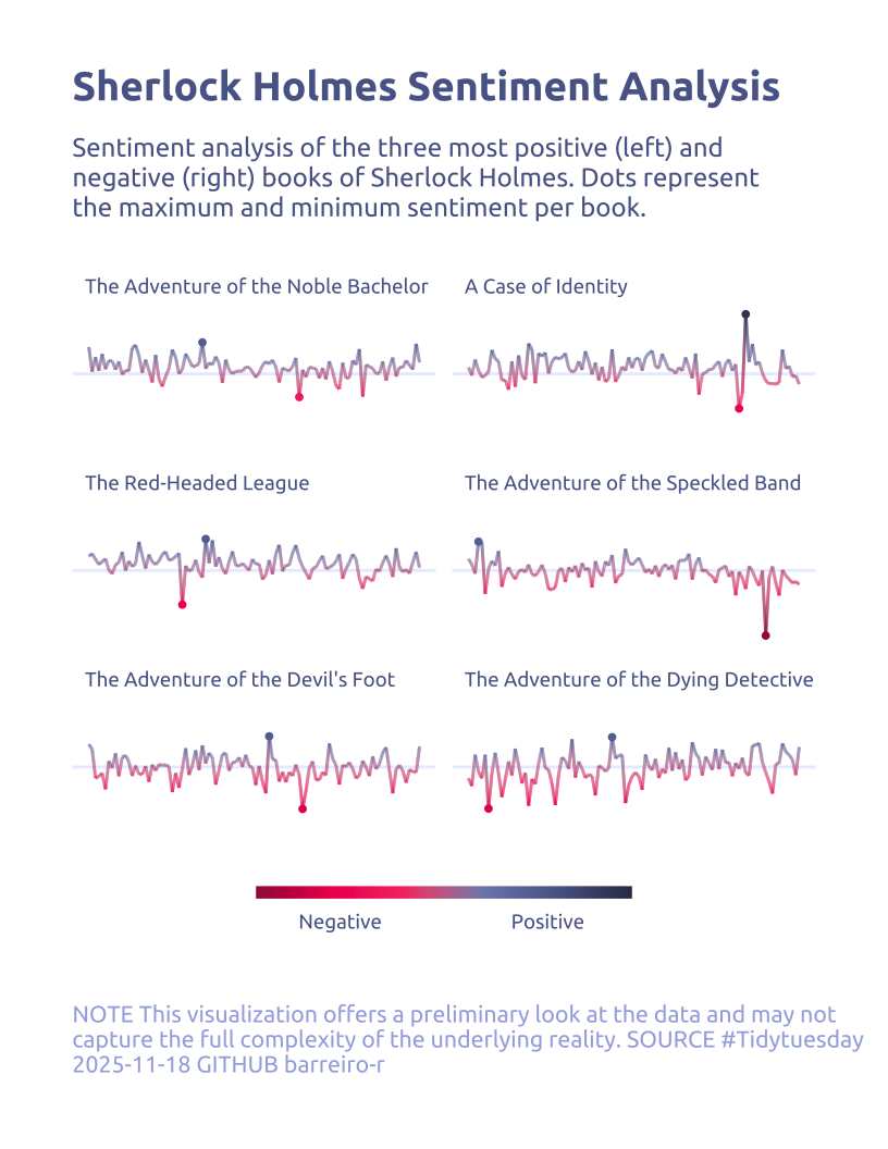
title = "Sherlock Holmes Sentiment Analysis",
subtitle = str_wrap(
'Sentiment analysis of the three most positive (left) and negative (right) books of Sherlock Holmes. Dots represent the maximum and minimum sentiment per book.',
width = 60,
) |>
str_replace_all("\n", "<br>"),
caption = str_wrap(
"NOTE This visualization offers a preliminary look at the data and may not capture the full complexity of the underlying reality. SOURCE #Tidytuesday 2025-11-18 GITHUB barreiro-r",
width = 80,
),
)